Pascal’s Diamond

The relevance of Pascal’s Triangle to a “best of seven” tournament, such as the World Series, is obvious. But there is that wrinkle of not actually playing all seven games. In the past I had contented myself with various adjustments, but I never actually drew up “Pascal’s Diamond”, which is based very simply on the same generating rule as the Triangle, but terminated appropriately, as shown here:
pascal1
Note that it’s equivalent to Pascal’s Triangle up to game 4 ( as indicated by the black numbers ) but terminates along the diagonals indicating 4 wins by either team. We immediately see that the nominal probability ( assuming “chance” outcomes ) of a 4,5,6, or 7 game series is 1/8, 1/4, 5/16, or 5/16, respectively.

Note that the equal probability of a 6 or 7 game series is a reflection of the “chance” outcome of game 6, which terminates the series at 4-2, or forces a game 7 with equal probability.

I decided to compare these probabilities with the last 91 world series results, in terms of games played, or equivalently, “games won by the series loser”. I found these to be 18, 18, 20, and 35. This compares to a nominal expectation of 11.37, 22.74, 28.43, and 28.43, for 91 “chance” games. So, this looks a little out of whack! But is it really? …

Oh No! Not STATISTICS!

Well, we don’t have to do a canned analysis, even if we find ourselves being driven that way. We can make up any sort of test and apply it experimentally to sets of 91 “chance” series, and determine the “probability of rejecting the null hypothesis”, in this case the hypothesis that the real outcomes obey the same statistics as “chance” would have it.

Let’s just try looking at a generated sequence of 91 chance-ruled series. Here’s 10 of them, with the average over all 10 at the bottom. Each row represents the number of 4,5,6, and 7 game series in a trial of 91.

$ series 10
9 20 31 31
9 18 38 26
12 19 32 28
14 14 37 26
12 20 31 28
12 19 33 27
12 24 32 23
11 23 27 30
11 25 27 28
8 26 26 31

11.000 20.800 31.400 27.800

Well, notice the 14, 14, 37, 26 … qualitatively very similar to the actual historical “trial” of 91 world series, so impressionistically, we don’t have grounds to believe the games are ruled by anything but chance.

I’ll just add that I did go “back to the books”, or Wikipedia as we do these days, and tutored myself on some of the sigma-based statistical tests, and I’m ready to report that it’s all very interesting!

The thing that wouldn’t stop

The “thing” is namely the “June 27th flow” ( that’s when it started ) of Kilauea on the big island of Hawaii. This flow seems unusual because it is a very thin tendril that has been “guided” by a long crack in the ground, forming an extended lava tube of about 10 miles length, as shown in this Sept 15 map. ( Click to enlarge. )
sept15
It looked for a while like it was headed for the Kaohe Homesteads, but then it spilled out of the crack and bypassed them, following the fall line of the land. Fall lines are shown on the map as blue lines, like streams. Now it looks like it is headed right for the town of Pahoa, which resembles a “shore town” in that it is pretty much built along a single thoroughfare, route 130. It’s projected to reach that road in about 10 days, and following the fall line it’s on, I see ground zero at this small block of homes, shown in Google Maps Street View.
pahoa
The official projection is something around there, but I couldn’t quite decipher it. It seems the only hope would be for it to stop, but it has been going for a month or so now and it’s hard to see that happening.

Here’s an animated gif view of the approaching “thing” in the form of a plume of smoke wending through the forested landscape. It’s a little hard to follow because the POV shifts backward as it advances. It starts as it advances along the “crack” and ends as it’s bypassing the Kahoe Homesteads.

output_TcItpr
UPDATE:
Here is the official projection of the flow into Pahoa.
sep17
It is very close to what I thought, which is after all just a matter of following the downward slope. Of course it remains to be seen if the flow itself follows this simple projection.

In the following Google Maps view, the street view I showed above is looking southwest along La’Au Place. The projected path in the satellite view is just south of that, on the other side of the grove of trees. Note the the dark rectangular roof visible in both views.
laAu
UPDATE Oct 24, 2014
After a seeming stasis, with little advance through most of October, the flow front has reactivated in the last few days: ( click to enlarge )
kilauea_Oct24
It has come within a few hundred yards of the “transfer station” ( a recycling drop-off ) on Apa’a St. on the outskirts of Pahoa, so it seems like some sort of incursion is imminent. ( click to enlarge )
multimediaFile-875
Update Oct 26, 2014
It didn’t take long for the flow to cross Apa’a St. (click to enlarge )
multimediaFile-896
It’s headed for the cemetery, of all things, and going down the cemetery road. Crossing this street has made the news, and brought out the comments: e.g. “What do you expect if you live on the side of a volcano.” Let us not focus unduly on the ignorance of the commenter. This is the way the news operates. Everything is in the abstract. Details are presented without context, so this sort of interpretation is to be expected. OTOH we may note that the presence of a cemetery on the line of flow suggests that this event is without precedent in living memory. A brief perusal of the maps of this flow backs this up. It is very unusual in its nature and its direction of flow.

Well, Kilauea is there, and I think the residents are duly philosophical about living next to it. It’s a very narrow flow, and they may have reason to hope that it will stay narrow as it cuts a path to the sea, and remain in the nature of a temporary disruption.

Update 10/29/2014

Are you superstitious ? I hope not … because I may be!

flow_oct29

Asteroid 2014 R6

Last March I posted NOTES ON CLOSE ENCOUNTERS, describing some thumbnail math relating to the hyperbolic shape of an asteroid trajectory passing near the earth, as viewed in the earth frame of reference.

I noted that the encounter with asteroid 2014 DX110 had a very “flat” ( high eccentricity ) trajectory, based on the speed and near approach distance of 1.3125 and 54, expressed in units of earth escape velocity and earth radius. ( Not earth orbit radius! ) The rule-of-thumb eccentricity came to 185 in that case.

The predicted encounter with 2014 RC set for this Sunday has a much less “flat” flyby trajectory, based on the available graphic shown here:

asteroid20140903-640

From the graphic we have, in terms of my previous post, r0 = 25,000 mi = 6.3 ; v0 = 40000 km/hr = 1 ( i.e. very nearly earth escape velocity. ) So this is a lot closer and a little slower than 2014 DX110. Turning to the formula

s2 = r02 / ( 1 – 1/ ( r0 v02 ) )

… we get an “impact parameter” ( projected asymptotic approach distance ) of 1.09 r0, so 2014 R6 will actually be “drawn” about 9% closer by earth’s gravity, compared to a straight line fly-by, and the hyperbolic trajectory has an eccentricity of 11, versus 185 and a deviation of just 1/2 % in the case of 2014 DX110.

Euclid & The Duchess


In Chapter IX of ALICE IN WONDERLAND Alice has a conversation with “the Duchess”, wherein the Duchess relates to her several “morals,” including the following:

“Be what you would seem to be”— or if you’d like it put more simply —“Never imagine yourself not to be otherwise than what it might appear to others that what you were or might have been was not otherwise than what you had been would have appeared to them to be otherwise.”’

It has occurred to me, and I feel firm in this, that Lewis Carroll meant this as a mock paraphrase of Proposition 6 of Book II of Euclid’s Elements:

If a straight line is bisected and a straight line is added to it in a straight line, then the rectangle contained by the whole with the added straight line and the added straight line together with the square on the half equals the square on the straight line made up of the half and the added straight line.

I forget the exact occasion, but it was as I was perusing Euclid that I was struck by the similarity of construction. The phrase, “straight line” , corresponds roughly to “otherwise” and “others” in the Duchess’ moral, and both expressions suggest a lilting meter. ( … and I hope I don’t have to remind anyone of Charles Dodgson’s mathematical vocation ! )

Furthermore, the syntax is similarly baffling, Euclid can actually be parsed, but not so the Duchess. Her moral contains three long phrases, each coherent on its own but with overlapping connections that make the whole thing incoherent:

Never imagine yourself not to be otherwise than what it might appear
to others …

it might appear to others that what you were or might have been was not otherwise than what you had been …

what you had been would have appeared to them to be otherwise.

However, note that Prop. 6 does contain a “garden path” , as described by Stephen Pinker in THE LANGUAGE INSTINCT.

This is the phrase, “the rectangle contained by the whole with the added straight line …” which one is inclined to take as a complete description of a rectangle. However, the following phrase, “… and the added straight line together with the square on the half … “ is rendered nonsensical if one goes down this path, because a line cannot be taken together with a square. Of course, (ahem) the phrase, “with the added straight line” refers to the base of the rectangle while, “and the added straight line” specifies the height.

To me, it all adds up, especially considering the preamble. “Be what you would seem to be” would stand for the algebraic expression:

(a+b)2 = a2 + 2 a b + b2 … OR … a ( a + 2 b ) + b2
… as per the theorem.  ( Note the “bee” and “two bee” in the moral. )

Also, “If you’d like to put it more simply”, alludes to the historically primitive character of geometry vis a vis algebra, which is somewhat more abstract. So Euclid’s book II may be construed as simpler than modern algebraic notation, being put in more primitive, or “simpler” terms.

Well, Heath was 40 years after ALICE, but I think that the english version of basic Euclid was probably already a matter of tradition by this point, although I really couldn’t say, of course.

NOTE ADDED IN PUBLICATION

All the above I’ve been carrying around for some years, but in anticipation of writing this up, I was spurred to check the original greek of Proposition 6:

… so feast your eyes! heh heh. Well, I spent some time on it but I don’t want to belabor the issue. You can note “tetragono” ( square ) and “gramme” ( line ) and “orthogonion” (!) orthogonal.

The thing I want to say about it is that the “garden path” does not exist in the greek, and the syntax seems to be a little more technical. “apo” means the base of a square, so it announces the specification of such, which is terminated by “tetragono” so that’s it, with no ambiguity.

The “garden path” clause specifies the base and height of a rectangle delineated by TO [ base spec. ] KAI [ height spec. ]

The base spec. is “upo tes holos syn te proskeimene” ( base of the whole with the extension ) and the height spec is “proskeimenes periexomenon orthogonion” ( encompassing orthogonal extension ? ) then comes “meta” = “together with” … ( the square on the half ) so there seems to be a more elaborate system of “terms of art” in play.

Consider a Spherical Square …

… of course I allude to the punchline, “Consider a spherical horse”, although there is such a thing as a spherical square. Namely a quadrilateral drawn on the surface of a sphere with equal sides and equal angles. Many years ago I was drawn into contemplation of this by a statement in Peterson’s Field Guide to the Stars and Planets, by Donald Menzel, that “The sky contains approximately 40,000 square degrees …” as excerpted here:
A more accurate value is given by 4Pi/(Pi/180) = 41252.96125, but this is still approximate, as it does not allow for the curvature of the “square degree” itself. So I endeavored to derive an exact value for the area of a spherical square degree, and did so, as recorded in this note:


I was quite pleased with this result at the time, as it was simple and even had a certain elegance, and in fact I had difficulty reproducing the calculation before I rediscovered my note. I did remember the result verbally: “four arcsine of sine squared alpha over two”, where alpha is the measure of the square across the center.

Applying this formula gives the value of 41254.00842 for “square degrees in the sky”, differing by about 1 in the units place from the linear approximation.

I recall that I knew at the time that the formula was “four arcsine of tan squared beta over two”, where beta is a side of the square. This gives 41250.86683, undershooting the linear approx. by about twice the amount that the alpha formula overshoots. I’m sure there’s a story there, but let’s move on.

I was recently drawn into contemplation of the spherical square by a NYT Quote-acrostic based on a quote by Calvin Trillin, which alluded to the infamous Indiana Pi Bill ( misattributing it to Texas ). The cited Wiki article offered in explanation of the bill’s content, a crank mathematical screed, that “it is clear that the assertion is simply that the area of a circle is the same as that of a square with the same perimeter”

I started wondering if this might not be true for some spherical square and circle. I finally realized that it is true of the “degenerate” spherical square whose sides are quadrants of an equator, but too late! … I was back on the case.

In my calculation, I had retreated to the comfort zone of spherical coordinates, and resorted to integral techniques which, while well within the bounds of Introductory Calculus, were less than straightforward.

I knew that the problem could be solved by methods of Spherical Trigonometry, but I didn’t see that these were any simpler.

Well, this time around I came up with a simple construction that makes it a “one step problem” , applying the rule of “spherical excess” for the area of a spherical triangle:

Well OK, a “two step problem”, we still have to solve for theta. This is an easy application of Napier’s rules for right spherical triangles applied to either the light blue or lavender auxillary diagram in the figure, and giving

or …

Additionally, we may solve for the distances x and y, which are the half-lengths of the sides of the spherical rectangle. Applying Napiers rules, as above, we get:

Note that when psi = chi and equivalently x = y, we have the identity

… as alluded to above.

Notes on Close Encounters

The passage of 2014 DX110 is just the latest in a series of  near earth encounters that have been observed, and it raises the question, what is the likelihood of one of these actually hitting the earth, supposing a continuing sequence of them? Of course this has been going on for a long time, and they DO occasionally hit the earth, but how might we model these encounters statistically?

Let’s take the lunar orbit standard and suppose that a medium sized asteroid passes within “the lunar hoop” perpendicular to its relative direction of motion, say once a year. Then if each of these objects has a constant probability per unit area of passing through a particular point in the hoop, we need only compare the cross section of the earth to the size of the hoop to estimate the fraction of these encounters that result in a collison with the earth, and this fraction is just the square ratio of the earth’s radius to the moon’s orbit, or about 1/602 = 1/3600 .

Gravitational Focusing

But then we might ask, what about the gravitational attraction of the earth? Wouldn’t it tend to “focus” objects passing nearby and increase the effective collision radius?

I think the answer is “somewhat”, but there is a simple treatment of the problem that is interesting more for the understanding it affords than any modification of such an estimate.

Let’s directly apply conservation of energy and angular momentum to get a simple and exact answer to the idealized “two body problem” of a small object passing by the earth in an inertial frame of reference. This is actually a reasonable approximation, I think.

Conservation of energy is expressed by

1/2 v2 – MG/r = constant

and conservation of momentum is expressed by

v rperp = constant

In particular, if an object approaches the earth from a great distance with speed v1 and s is its projected straight line distance of closest approach ( measured to the center of the earth, ) then its angular momentum wrt the center of the earth is v1 s , and if r0 is the actual hyperbolic distance of closest approach, where it has velocity v0, we must have

v1 s = v0 r0

A hyperbolic Interlude

The situation is illustrated in the following diagram, which shows the hyperbolic path of an object passing the earth ( in blue ) and the asymptotes of the hyperbola in gray:

The diagram has been drawn to scale for a hyperbola with parameters a=7, b=24, which gives the focal distance of sqrt( 72+242 ) = 25, and hence the rational eccentricity of 25/7 . It’s part of a sequence of pythagorean triples with the lowest element being the sequence of odd integers beginning with three, and the two larger elements differing by 1 ..

3 4 5
5 12 13
7 24 25
9 40 41

This is of purely heuristic interest, but it gives us a sequence of “rationalized” hyperbolas with linearly increasing eccentricity.

Note that our ratio of interest, s/r0 , is also rational. 7 24 25 is the 3rd entry in the list, and the generalization holds that this ratio is (n+1)/n for the nth entry. We’ll come back to this …

Dynamics continued

We can simplify our notation by an appropriate choice of units. We note that the formula for conservation of energy, with constant set to zero :

1/2 ve2 – MG/re = 0

or

1/2 ve2 = MG/re

… is the defining equation for the escape velocity from the surface of the earth, and we can express the potential energy in terms of the escape velocity:

MG/r0 = 1/2 ( re / r0 ) ve2

Then if we measure r in units of re, and v in units of ve, Conservation of energy between the far motion at velocity v1 and zero potential energy, and the close approach v0 can be simply expressed as:

v12 = v02 – 1/r0

Note we have “multiplied through by 2” to get rid of the factor of 1/2 in each term.

Now we can use the equation for conservation of angular momentum to express v0 in terms of v1, or vice versa, and with some elementary rearrangement of terms we get these two equations for s in terms of r0 and v1, or r0 and v0 :

s2 = r02 ( 1 + 1/ ( r0 v12 ) ) = r02 / ( 1 – 1/ ( r0 v02 ) )

Notice that for large v1, i.e. much greater than earth escape velocity ( implying large v0 as well,) we have r0 = s, so the object just zooms right by. Otherwise, we have an easy formula for determining s in terms of r0 and v1 or v0 .

Impact criterion

If we set r0 = 1, i.e. the radius of the earth, we have a very simple formula for the apparent or effective size of the earth in terms of v1, expressed in units of earth escape velocity.

s = sqrt( 1 + v1-2 )

For example, for the earth to “appear” twice its diameter, the incoming speed would have to be 1/sqrt(3) = .58 , or 58% of earth escape velocity.

The case of 2014 DX110

Well what about 2014 DX110 ? It’s stated that its flyby speed was 33000 mph or 14.7 km/sec, compared to 11.2 km/sec, so v0 = 1.3125

It came within 54 earth radii at close approach meaning r0 = 54, and we can use the v0 version of our formula to get

s = 54 / sqrt( 1 – 1/ ( 54 x 1.31252 ) ) = 54 x 1.0054

s/r0 = 1.0054

… and finally

To find a rationalized hyperbola which “approaches” this case, we note ( as per above ) that (n+1)/n = 1 + 1/n, so we want n = 1/0.0054 ~= 185, so we take the 185th in the sequence of Pythagorean triples:

371 68820 68821

and eccentricty e = 68821/371 ~= 185.5

Sol 550 : A MAHLI Panorama

Here is a hotlinked sol 549 Navcam image of a small ridge that captured the interest of Curiosity. I think it’s about 2 feet long:

On sol 550 it took a series of MAHLI closeups, and also this Navcam image of the robotic arm ( with the MAHLI on it ) during the process of doing so:

BTW, here is an image which shows the arm in the stowed position, prelaunch:

There are three joints on the arm itself, with all the axes parallel, so it moves in one plane with motion of these three joints. There’s a vertical “post” that carries the arm assembly and allows it to swing out and away from the base. You can see it projecting downward near the left front wheel.

You can also see the name plate on top of the upper beam of the stowed arm, and the forward projecting arm joint at the right side of the rover. These are visible in many of the downward looking Navcam and Mastcam images, including the first image of this post.

If I had understood all this correctly, I never would have made that blooper in my SPOT OF BOTHER post!

Anyway, the MAHLI took a series of images of this little ridge on sol 550, and they appeared to be suitable for a panorama, so I tried it. It worked pretty well, but it is not a true panorama. The images on the left were part of a “scan” where the MAHLI changed position but kept pointing in the same direction, more or less. Then the images at the right were made by swinging the POV outward. It stitches down the centerline pretty well, but you can see some doubling up of particular features above and below. Well, a nice result and it shows incredible detail. As always, CLICK TO ENLARGE!

Mandelbrot II : Julia Islands

I mentioned the image gallery section of the Wiki Mandelbrot Set article as the starting point for my renewed interest in this topic. It is based on a zoom sequence terminating on a “Julia Island”, which is a component of the Mandelbrot set resembling a “Julia set”, which is based on the actual sequence of an iteration rather than the in/out criterion of the Mandelbrot set. So there’s a little math magic in this resemblance.

Here is my recreation of the zoom, based on the linked tool I mentioned, which by no means outstrips the images in the article ( which can be expanded, ) but it does go a little deeper, and it keeps the Julia Island location at center. This was easy to do by working backwards from the deepest image and keeping the same coordinates by simply changing the scale in the URL field.

Here’s a “hot link” of the lowest level of the Wiki zoom :Wikipedia commons( To see its full glory visit the site. ) It roughly corresponds to the antepenultimate frame of the animated gif. The commentary in the main article notes that there is a “satellite” ( i.e. “mini-Mandelbrot set” ) at the center of the island structure that is “too small to see at this magnification”. Just visible there is the large square structure in the center of the last frame of the gif, where you can almost see the satellite at the center of it, as a tiny dark speck.

This conclusion is supported, if not confirmed, by perusal of a nearby and entirely analogous structure, which is a little bit larger. Here’s a slower zoom, taking 1/2 per frame instead of 1/10, showing a descent through the analogous square structure to reveal the Mandelbrot satellite.

Note the emergence of a new “sea” of similar spirals and structures as part of the INFINITE descent. It’s fascinating and incredible and, like the song says, “a little bit frightening.”

Looking back at Dingo Gap

Here is a 3 X 4 panorama from Mastcam images acquired on sol 538 around 2014-02-09 22:37:19 UTC. (Click to enlarge ! )

Compare the near horizon with this view from the landing site on sol 3:

You can see the same mesa-like structures on the lower reaches of Mount Sharp, and the same low dome to the left of them. Note that the gap between the mesas has opened up from the new position, as Curiosity has moved back and to the right from this sol 3 POV.

Finally, this animated gif is from the Rear Hazcam on sol 538, with images acquired at 2014-02-09 22:03:32 UTC, 2014-02-09 22:56:48 UTC, and 2014-02-10 00:37:23 UTC, so the second of these seems to be the POV of the Mastcam panorama. Note the dome of Mount Sharp visible in the first frame. … A very nice shot!

The Mandelbrot Universe

I recently saw one of several “Deep Zoom” videos of the Mandelbrot set, which I’ll leave alone for now, but it got me interested in the subject, which I haven’t thought about since the 1980’s. Times change, and the facilities available for investigating the subject are now, of course, much more powerful. I looked at the Wikipedia article on the Mandelbrot set, which refreshed and greatly expanded my casual knowledge of the subject. The exciting thing though is the link under the section headed “Image gallery of a zoom sequence” to an “interactive viewer” ( go to Wikipedia to get the link. ) It indicates it will open for “this location” ( i.e. the one illustrated ) but I found it goes to the initial full view of the set.

Anyway, it’s a fabulous tool. You can click on a spot to zoom by a factor of two, and although it does take time to calculate the image, you can click again for repeated zooms without waiting for the full resolution. I found it very handy to use. It goes down to 10^-14 in scale, which is well short of the claims made by these deep zoom videos, but it provides ample scope for casual exploration.

Note the parameters are passed in the URL address field, and these can be edited and entered with the naturally hoped for result. Of course you can save them and reenter them to bring back the image, so as I say, very handy.

I also used the extended precision calculator, bc, on Cygwin to explore some of the mathematical aspects, which I’ll get to. First, here’s an animated gif of a short zoom on a large portion of the Mandelbrot set, progressing down the scale of the circular “bulbs” along the real axis. This is a more extensive version of the “Mandelbrot zoom” gif in the Wiki article which uses a loop of two circles without “hair”.

First note that the Mandelbrot set itself is the black area, determined by points c, where the iteration of the defining formula always remains bounded. The “hair” is exterior to the set and is colored according to how rapidly the formula diverges under iteration.

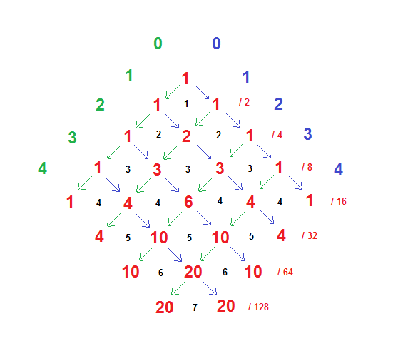
These circles are in the set, and are called “period bulbs” in the article, because of the defining nature of the points within them. That is, they are points c, in the imaginary plane, such that iteration of x = x^2+c ( where ‘=’ means assignment, as in a programming language ) starting with x == 0 ( ‘==’ asserts equality ) converges to a cycle of fixed values, these values being 2 in number in the “2” bulb ( the first circle ) then 4 in number, then 8, 16, 32, and 64 in number in the large circle of the sixth and last frame.

This brings us to the math, and bc. Let’s go for the gusto with the “64 bulb”. Using the “click and zoom” facility in the interactive viewer, we go to the sixth bulb, i.e. the 64 bulb, and simply copy and paste the x-axis ( i.e. real part ) value into bc, and initialize x to 0:

c= -1.400968738408754
x=0

Then we iterate for a goodly number of times to assure ourselves of convergence to a stable cycle, in the belief this must happen:
( Even though bc runs interpretively, the power of a modern PC is such that this number of iterations causes a barely perceptible hitch in the response )

n=100000
for( i=0 ; i<n ; i++ ) x=x^2+c;x
.010561399880314

Now we check for a 64 cycle of values:

n=64
for( i=0 ; i<n ; i++ ) x=x^2+c;x
.010561399880314

OK! But maybe this is a repetition of a shorter cycle, so check 32:

n=32
for( i=0 ; i<n ; i++ ) x=x^2+c;x
-.000137388541270
for( i=0 ; i<n ; i++ ) x=x^2+c;x
.010561399880314

OK again!  We can now be satisfied that 64 is the true cycle value. Note that we didn’t use a lot of precision, but the “attractive cycle” is strong medicine, and we don’t need it. We are just checking the fundamentals though, and of course there are more delicate arrangements to be found.

In particular, what about the “vanishing point” of this self-similarity? It is cited in the article to crude precision as -1.401155, which can be discerned numerically, but what are its defining properties? This point remains obscure to me.

Misiurewicz points

These are defined as values of c such that k iterations of x=x^2+c give a value that repeats after n ( more ) iterations, and are designated as M_k,n, and these form vanishing points for self-similar transformations although they do not account for the seemingly fundamental one just described. Noteworthy is M_4,1  described in the Wiki article.

Here is a zoom which goes by steps of 100X magnification ( after an initial step of 10X )
The Wikipedia article on Misiurewicz points mentions … “(Even the `principal Misiurewicz point in the 1/3-limb’, at the end of the parameter rays at angles 9/56, 11/56, and 15/56, turns out to be asymptotically a spiral, with infinitely many turns, even though this is hard to see without maginification.)” ( sic ! just noticed that. ) … This is our guy, and you can see the “slow roll”, which advances by about 50 degrees in 6 steps of 100X magnification. ( I’m still working on the meaning of those angle values. )

In this case we can do a little math and come up with a way to define the M_4,1 point, at the center of the zoom, to arbitrary precision. Approaching it graphically we see the center at approximately ( -.10109636 , .95628651 ) in the complex plane.

In bc we define functions:

define f(a,b){ return( a^2-b^2 + c); }
define g(a,b){ return( 2*a*b +d ) ; }

… which are the real and imaginary parts of the formula, x^2 + (c,d) , applied to a complex value x with real and imaginary parts (a,b) . So we can proceed to apply the formula iteratively and see if we come up with a constant value after 4 iterations, as per the M_4,1 designation:

c= -.10109636
d= .95628651
x=y=0
z=f(x,y);y=g(x,y);x=z;x;y # iteration 1
-.10109636
.95628651
z=f(x,y);y=g(x,y);x=z;x;y # iteration 2
-1.0053597752027305
.7629323394437928
z=f(x,y);y=g(x,y);x=z;x;y # iteration 3
.32758616302650612570470420629841
-.57775646055620961839245967248080
z=f(x,y);y=g(x,y);x=z;x;y # iteration 4
-.32758619350801035155822390304043175425331545129536
.57775646584523271983382407623684575759993010598581
z=f(x,y);y=g(x,y);x=z;x;y # iteration 5
-.32758617964890595894029463234712218921204878613363
.57775642715823884156305664636678518208809205705010

Note that the 4th iteration approximately achieves the repeated value, but the 3rd iteration is the negative of it. So to home in on the exact value we want to adjust c so that f(f(f(f(0)))) = – f(f(f(0))). Without spelling it all out, we can do this by numerically evaluating the sum of the 3rd and 4th iterate ( which we want to be 0 ) to see how it varies with small variation in the real and imaginary parts of c . This is essentialy “Newton’s method” of finding roots. Inverting a simple 2X2 matrix tells how to vary ( c, d ) to bring this sum to 0. By iterating this estimation we can find  the correct complex value of M_4,1 to arbitrary precision.

Here’s as far as I’ve taken it so far:
( c, d ) = (
#real part
-.1010963638456221610257854457386225654638054428262534
838769311776607808407404705842748212198105167791
,
# imaginary part
.9562865108091415007710960577299774358098333365105291
700343143215005246590657167325269784107873398073
)

It’s very easy to do and could be taken to many thousands of decimal places in less than an hour, I’m sure.

I’ve got a lot more, but I want to put something out now and I do plan to continue my discussion … but let me just outline my thoughts.

The mathematical structure of the Mandelbrot set has been a matter of ongoing investigation, and is a difficult subject. One fundamental point is the “connectedness” of the set, and it has been proven that it is “connected” according to the literature. Well, I’m sure it has, but I still have questions! In particular it seems to me that these Misiurewicz points must be isolated elements of the set. Perhaps in some sense they are, since topology has more definitions than you can shake a stick at.

Anyway, I hope to be back with more pictures.