Spherical Trigonometry is used as a gateway to abstract mathematics because it can be taught as the study of the  geometry of  an intrinsically curved surface, without reference to its embedding in a “flat” 3-d space, as we experience it. So this is the preferred and usual method of teaching.

Still, I found myself a bit unsatisfied when I recently looked up, for study, the Spherical Law of Sines, which stands in direct analogy to the Law of Sines of plane trigonometry, with one important variation. That is, the sides, a and b, as referenced in the latter, become sin a and sin b in the former … very mysterious!

I found that the proofs tended to be algebraic in nature, depending on various “trigonometric identities” and I wondered if I couldn’t come up with something a little more “concrete” using constructive methods of traditional spatial ( Euclidian ) geometry.

So, doodling around, I found that I had great difficulty visualising 3-d constructions by reliance on 2-d diagrams, i.e. drawn on paper.

So I decided, well, I’ll make a model out of wood.

Of course, that requires a little doing. The obvious method is to cut out a sector of a sphere along central planes, but that isn’t exactly easy, and it wastes most of the sphere ( even if you can make several this way from one sphere. )

Also, wooden craft or carving balls are expensive, and usually rather small. So I decided to cut one from a block. I could buy a bag of 8 or 10 suitable blocks for a few dollars, and I could use two of the flat sides for the plane surfaces of the defining central planes. This would give me a nice RIGHT spherical triangle, while minimizing the carving effort.

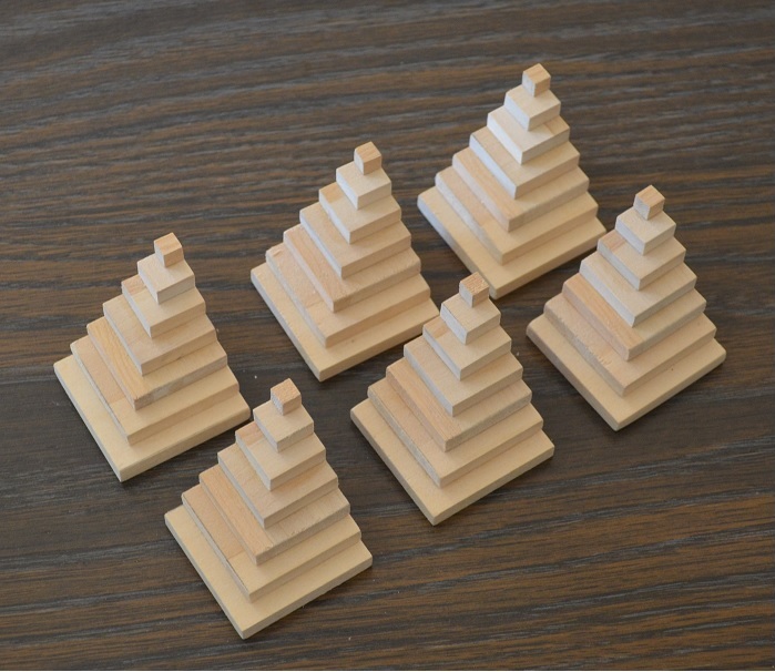
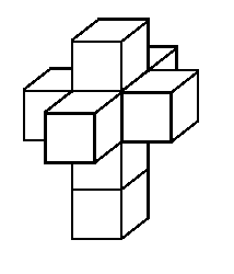
So, here is the completed result, along with another block showing the preliminary mark-up:

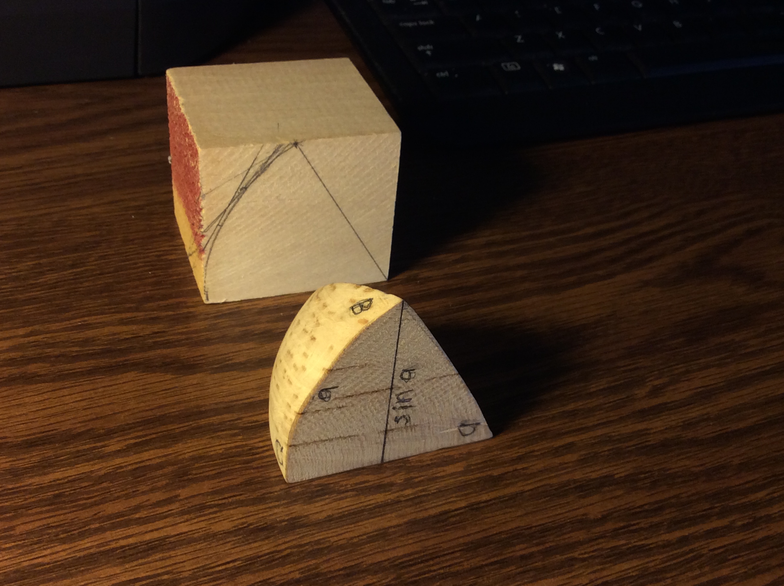
BTW, forming the curved surface wasn’t as laborious as I thought it would be. I could get reasonably close by cutting easily defined tangent planes to the surface, and then sandpaper made short work. Of course, it’s not perfect!

Napier’s Rules and the Spherical Law of Sines

Well, I had already noticed that the Spherical Law of Sines could be reduced to one of Napier’s Rules, in this case (R2) as named in the Wikipedia article on Spherical Trigonometry.

(R2)      sin a    =   sin A   sin c

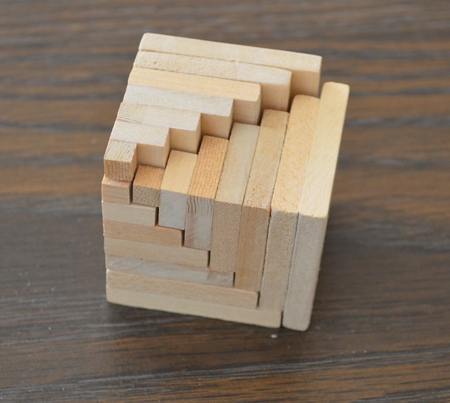
In the image below, angle A is at the base of the spherical triangle at the top of the photo, and measures the dihedral angle at bottom right. So it’s a simple application of “opposite over hypotenuse” to see that   sin A = sin a / sin c , which is (R2) above.

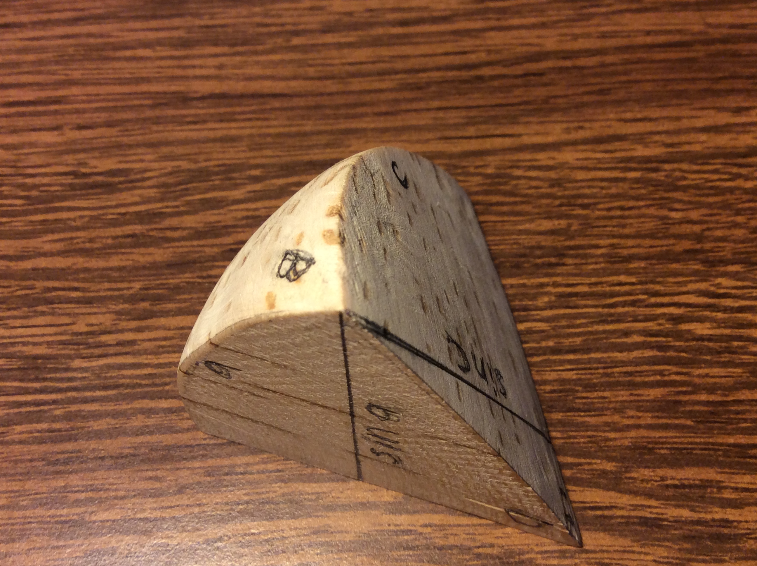
Note also that sin a and sin c are defined by the central angles, a and c, which measure the sides, a and c,  of the spherical triangle.

To get the Spherical Law of Sines all that is required is to place next to it another right spherical triangle sharing side a, along with the perpendicular plane face subtending it, to form a “general” triangle.

The shared altitude, sin a, then plays the same role in the proof as the shared altitude used in the proof of the Plane Law of Sines.

… and that’s all I have to say about that.

The Hot-wire Foam cutter and the Spherical jig

Now for the really fun part:

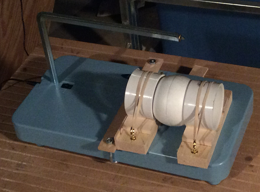
This is a hot-wire foam cutter equipped with a “spherical jig” of my own devising. As you can see it holds a 3″ foam sphere to be cut in half ( as adjusted . )  By cutting the same sphere in half  “three  ways”, I can form a spherical triangle along with its subtending solid central angle, just like the carved wooden model above.

Of course, I automatically get 8 such triangles. In the general case these will be 4 distinct triangles, along with their mirror inverses.

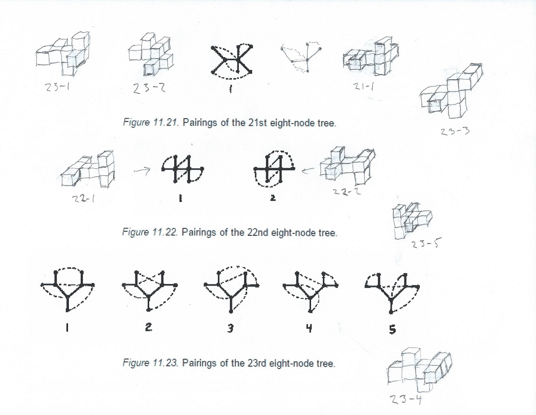
A Spherical Zoo

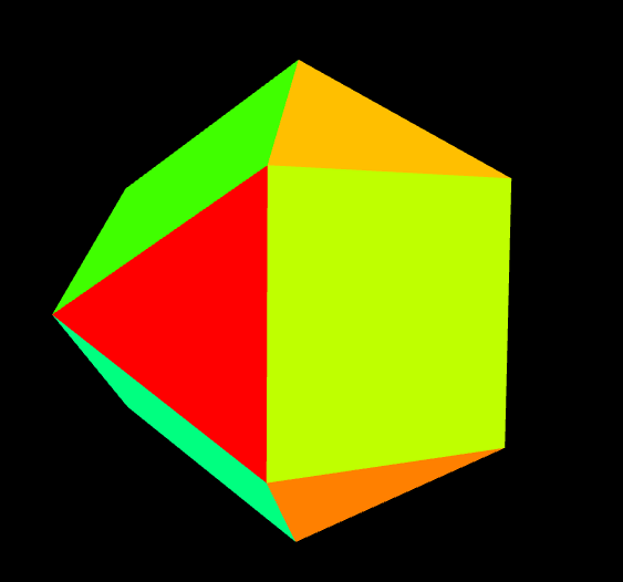
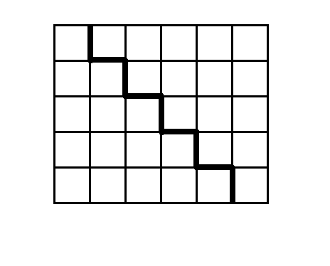
Here’s a “special” case of a such a production, contrived to produce a “large” equilateral triangle ( of course two of them ) and whatever else “falls out” :

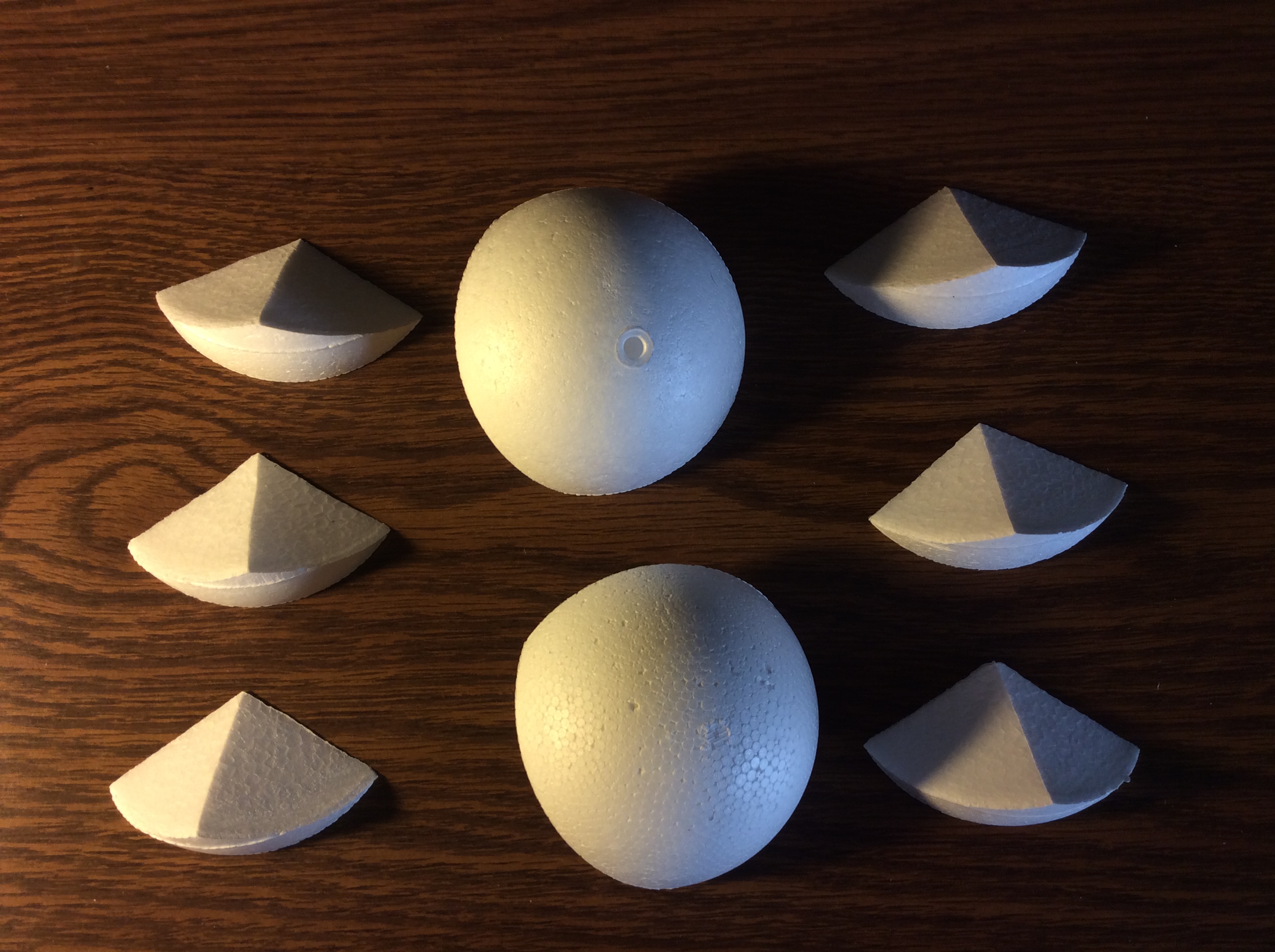
The “large” equilateral triangles, inverses of each other, but in this case identical, are in the center.

Then six identical isosceles triangles are arranged on the sides. These form an equatorial ring between the two polar equilateral caps.

I first thought that this accounted for all possible isoceles triangles, but these are just a subset. They are the isoceles triangles which have the length of each ( equal )  side as the supplement of the base. That is, the base plus one side equals a 180 degree arc.

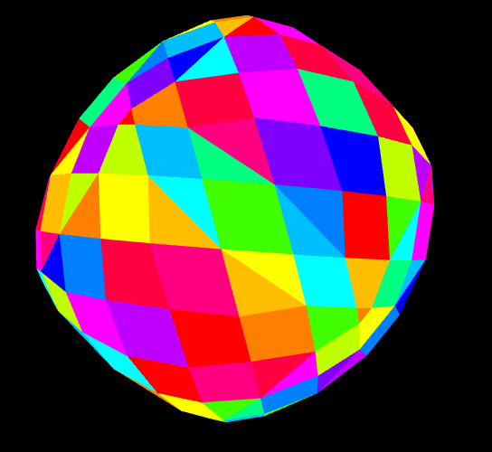
Just part of the arrangement that I think of as the Spherical Zoo.

Some “Nuts and Bolts”

I had been pondering how to organize this Zoo, and I was thinking in terms of the edges of the triangles of a partitioned sphere. This seems natural, since a “small” triangle can have arbitrarily short edges, just like plane triangles.

However, the triangles of a partition can also be specified by their ( corner ) angles, and this has the advantage that we can use the “spherical excess” rule, which gives the area of a spherical triangle in terms of the “excess” above 180 degrees, or “pi”. In fact, the area, in units of R squared, regarded as “Unity” for a given sphere, is exactly this value, expressed in radians.

So, using this scheme, I came up with a simple “map” of all the possible divisions of the sphere into triangles, in terms of A, B, and C, the angles of any one of the 8 triangles in such a division.

Well, with regard to units, we can have our cake and eat it too by specifying these angles in terms of pi/180 radians, which corresponds to “degrees”, but reminds us that the area is measured in “steradians”, of which there are 4 pi to be accounted for among the 8 triangles of a division, using the spherical excess rule. Note that this is nothing to do with “square degrees” … which we won’t touch.

In fact, since our “degree” is pi/180 radians, the 4 pi steradians  of the sphere are measured by 720 degrees, or 720 X pi/180. I explain all this so that we can do examples with angles, and areas, expressed in small integers. That this is possible is remarkable in itself!

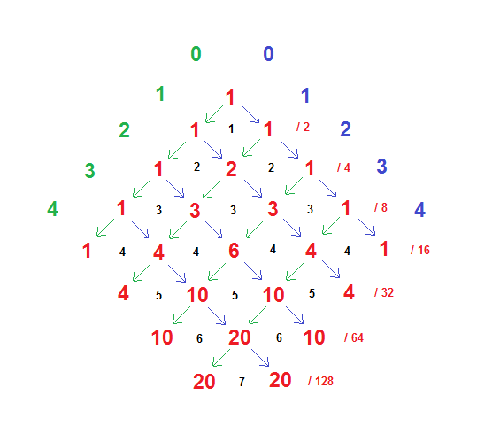
… so then my “map” :

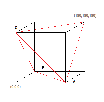
… The angles A, B, and C , with values 0 thru 180, as indicated, will specify a valid spherical triangle whenever they are the coordinates of a point lying inside the tetrahedron drawn in red.

Very simple!

… to be continued

On what basis I don’t recall, I was led into the contemplation of the generalized process of “cuboctization” which produces the cuboctahedron from the octahedron. This process is namely the connection of the midpoints of “neighboring” edges, to produce a new figure with vertices at these midpoints, and with the constructed edges.

It’s important to note that this figure, being composed of vertices and edges, is not necessarily a geometric solid, since the new vertices may not lie in a plane, to form a face. Nevertheless, we may proceed.

Of course the founding idea is the production from the octahedron

of the cuboctahedron, which may be regarded as a truncation of the octahedron, but in this case can be regarded as being produced in the manner described.

So we may proceed in this manner, and to arrive at the nub of the discussion in short order, we may present “cubocta5”, the result of applying the algorithm of edge midpoint connection four more times.

But here we have run aground. You can see that the four expected quadrilateral faces next to the green quadrilateral face in the center have been “bent”. Their defining vertices did not lie in a plane. We may remind ourselves that our procedure did not have any reference to faces at all, but only vertices and edges, so that we were only lucky up to this point to produce flat, or planar, four sided faces.

… but it’s close! So, what to do? Can we “flatten” these faces somehow, and produce a true cubocta5 polyhedron?

Never fear! A way was found. By retreating to the cubocta2, and adjusting the position of the vertices, we produced this version

All on a hunch, if you will. But that’s not half the story! At any rate, three iterations of our edge production algorithm produce the desired result. A truly remarkable figure with 192 vertices, 384 edges, and 194 faces. 8 of these faces are small triangles at the corners of a cube, and the remainder are quadrilaterals of varying proportions, but all perfectly flat.

If this figure “exists in the literature”, we would like to know, but at any rate, this version of it is original with us.

Some Numerology

It’s additionally remarkable that the entire figure can be specified in terms of small integers for the coordinates of the vertices, and there are only six distinct vertices required to produce the entire figure under octahedral symmetry. Here they are with the number of replications:

(24) 10 6 0
(24) 12 2 0
(48) 11 4 2
(24) 8 8 2
(48) 9 6 4
(24) 7 7 6

The 48 replications are the 6 permutations of the values times the 8 versions of each obtained by taking +/- each value, in combination.

since +/- 0 = 0, there are only 4 sign combinations for 10 6 0 and 12 2 0, and in the case of 8 8 2 and 7 7 6 there are only 3 distinct permutations, times the 8 sign combinations. Of course these add to 192.

Because … just look at the guy!

Looks like a regular barrel of monkeys!

He is the namesake of Faulhaber’s Formula, although he did not formulate it, as Wikipedia points out, but he more than laid the groundwork, I think anyone would agree.

Unbeknowst to myself, I had been following in his footsteps ( a very short way, of course ) in my pursuit of mathematical diversions. His namesake formula is a generalization of the idea of finding a formula for the sum of integers, from 1 to N, each taken to a given power. Familar to many is the formula for the sum of integers, i, from 1 to N, which is remembered as “first plus last times n over 2” or with these fixed limits, N(N+1)/2 .

I had presented this rule in graphical form as :

Showing an N by N+1 rectangle divided into 2 pieces, each representing
the sum of 1 thru 5.

So, I had the thought of representing the sum of the squares of integers in like manner, and made these model pieces.

I originally made 3 pieces, and noticed that these fitted readily into the following form, noting that there is a left handed and a right handed version, even though each piece is mirror-symmetric:

So then with due attention to “handedness”, ( do we need same, or opposite ? … ) we get this result:

Noting that the bottom square of each piece is N x N, with N=7 in this case, you can see from the picture that the block thus formed is N x ( N + 1 ) x (2 N + 1 ), so 1/6 th of this value gives the sum of integers from 1 thru N, each squared.

Moving right along

All this transpired some time ago, and I don’t believe that I got as far as the name of “Faulhaber” at that time, being content with my “physical derivation”. Just lately I pursued the issue a little further, going as far as N=3 and N=4, using simple algebra, much as Faulhaber must have done in some form or another, although he went all the way to N=17.

My method was to assume a formula, e.g. for N=2, of the form sum_1_to_N(i^2) =
a N^3 + b N^2 + c N + d , and then require that, sum( (i+1)^2 ) – sum( i^2 ) = (i+1)^2. It’s all just bookkeeping and I got the required answer, then I went to N=3 and did the same thing, and “discovered” ( for myself ) the “well known” result that the answer is simply ( N(N+1)/2 ) ^2 … amazing! I never knew!

Flushed with excitement, I realized that this lent itself to a simple 2-d graphical representation, which I worked out easily, and here it is:

Looking at the left and bottom edges, you can see the sequence of 1 2 3 4 5 6 7, in alternating colors, which immediately gives the “squared” result for the sum just cited.

Then looking at the red bands, you’ll see that these contain, in sequence, 1 1×1 square, 3 3×3 squares, 5 5×5 squares, and 7 7×7 squares, representing the cubes of the odd numbers. The blue bands represent the cubes of the even numbers in the same way, except that one square is split into two identical rectangles at each edge, a necessity required for an even number of squares.

So there it is! I don’t know where else you might find this kind of diagram, but this one is my own production, at least.

Of course, this is a followup to my previous post, but it merits a separate entry, I think.

It was only natural that I would want to push ahead to 6 from 5, but to do so, I abandoned my application of the “pivot principle” for a more simple and predictable “aufbau” technique, in which we add the 12 component 5-cubes one by one to build up all possible connected subsets of 2, 3, 4, …, 12 of which the last represents the possible unfoldings.

The simple principle is that all cubes are equivalent among the remaining pairs where neither member has been added. This limits the combinatorial excess of multiple versions of equivalent configurations under the symmetry operations of the 6-cube. These operations are the 6! reorderings of the axis labels times the 2⁶  “flips” of the axis orientations, amounting to an impressive 46080 operations.

This number is what creates the time bound for the complete calculation. It took only 4 seconds to generate  2499470 candidate configurations of 12 cubes from the unique canonical representations of the 11 cube configurations:

$ time build1 < cube11 | wc -l
2499470

real 0m4.174s
user 0m4.085s
sys 0m0.124s

… however it took over 8 hours to reduce each of these to its canonical value, requiring just another minute for the final step:

$ time sort -u cube12.canon | wc -l
502110

real 0m28.491s
user 1m37.750s
sys 0m0.310s

…  Of course, I saved the result in a file named cube12 , which has the “grep format” explained in my previous post:

$ head cube12
….00 ….01 ….10 …0.0 …1.0 ..0..0 ..1..0 .0…0 .1…0 0….0 1….0
….00 ….01 ….10 …0.0 …1.0 ..0..0 ..1..0 .0…0 .1…0 0….0 1….1
….00 ….01 ….10 …0.0 …1.0 ..0..0 ..1..0 .0…0 .1…0 0….0 1…0.
….00 ….01 ….10 …0.0 …1.0 ..0..0 ..1..0 .0…0 .1…0 0….0 1…1.
….00 ….01 ….10 …0.0 …1.0 ..0..0 ..1..0 .0…0 .1…0 0….0 1..0..
….00 ….01 ….10 …0.0 …1.0 ..0..0 ..1..0 .0…0 .1…0 0….1 1….1
….00 ….01 ….10 …0.0 …1.0 ..0..0 ..1..0 .0…0 .1…0 0….1 1…0.
….00 ….01 ….10 …0.0 …1.0 ..0..0 ..1..0 .0…0 .1…0 0….1 1…1.
….00 ….01 ….10 …0.0 …1.0 ..0..0 ..1..0 .0…0 .1…0 0….1 1..0..
….00 ….01 ….10 …0.0 …1.0 ..0..0 ..1..0 .0…0 .1…0 0…0. 1…0.

$ tail cube12
….00 …0.0 …11. ..0..1 ..0.1. .0…1 .1.1.. .11… 0..0.. 00…. 1.1…
….00 …0.0 …11. ..0..1 ..0.1. .0…1 .1.1.. 0…0. 0.1… 1..0.. 10….
….00 …0.0 …11. ..0..1 ..0.1. .0…1 .1.1.. 0…0. 00…. 1..0.. 1.1…
….00 …0.0 …11. ..0..1 ..0.1. .0…1 .1.1.. 0…0. 01…. 1..0.. 1.1…
….00 …0.0 …11. ..0..1 ..0.1. .0..0. .1.0.. .11… 0..1.. 0.1… 10….
….00 …0.0 …11. ..0..1 ..0.1. .0..0. .1.0.. .11… 0..1.. 00…. 1.1…
….00 …0.0 …11. ..0..1 ..1.1. .0…1 .1..1. 0…0. 1..0.. 1.0… 11….
….00 …0.0 …11. ..0..1 ..1.1. .0…1 .1.1.. 0…0. 00…. 1..0.. 1.1…
….00 …0.0 …11. ..0..1 ..1.1. .0..0. .1.0.. .10… 0..1.. 00…. 1.1…
….00 …0.0 …11. ..0..1 ..1.1. .0..0. .1.0.. .10… 0..1.. 1.1… 10….

VISUALIZING THE 6-CUBE

OK, there are 502110 canonically unique unfoldings of the 6-cube into 5-cubes, but what does this even mean? Can we picture it in any way? I think we can! Although 6 orthogonal axes are a challenge to ones powers of visualization. Here was a first attempt at it:

I should note that this is an example of Oblique Projection, which allows great latitude. Essentially, one can pick a “star” of any six line segments as representations of the six orthogonal unit vectors, with the only requirement being that each edge is represented by a parallel displacement of one of these.

Well, we can see that there are four tesseracts there, connected in a ring, but it really has the appearance of a “rat’s nest” and it does not make an attractive working model.

Much better is the idea I had of a “cubed cube” – a large cube whose corners are each split into a small cube whose vertices inherit the connections of the large cube. This is really just a refinement of the above, but a big improvement:

Now we come to the step of finding 5-cubes to use as building blocks for the unfoldings, and it just falls into our lap! There are six each of two varieties of 5-cubes evident. We will choose one of the six “cubed” faces of the large cube:

It is a “cubed square”. Can you see the other six 5-cubes? They each consist of 8 corresponding faces of the small cubes, connected by four large cubes, one at each corner. We needn’t worry about them, though, because all we need is the one we have, and all connections of the unfolding are made by parallel displacements along the 5 axes.

The two axes forming the large square provide a representation of the planar unfoldings of the 3-cube, with the connections formed by the overlap of the “edges” ( which are tesseracts. ) The other three axes are the axes of of the small cubes, which stack ( four at a time ) face to face to form a representation of the cubic unfolding of the tesseract.

Taken together, these comprise 5 independent lines of connection, but the split into a 2-d plus a 3-d component makes the job feasible as a manual step-by-step process using MS paint. Here is one result, arbitrarily produced:

This is 178th in the sorted list of 502210 canonical unfoldings. It’s early appearance can be accounted for by the simplicity of the scheme used, which relies exclusively on direct opposition of pairs.

178: ….00 ….01 ….10 …0.0 …1.0 ..0..0 ..1..0 .0…1 .1…1 0….1 1….1

Maybe somebody’s already done this, but not as far as I know!

The Wikipedia Tesseract article has a link to a 1984 article in the Journal of Recreational Mathematics, Unfolding the Tesseract . I had come upon this by following a circuitous path starting from a new NYT Sunday Magazine puzzle which involved tiling a small grid into “islands in an ocean” according to certain rules. This led me into unfoldings of the cube because a few years ago I had “discovered” a simple unfolding which very easily “tiled the plane” with simple translations.

So I looked into unfoldings of the cube and came upon the generalization of the idea in the form of the above cited article, which enumerates with hand illustrations the 261 unique unfoldings of the tesseract, based on topological reasoning.

I found the article to be fascinating, but I had to think about it a while to see how this seemingly abstract reasoning connected to the actual block models of these unfoldings, but I think I mastered it, at least in intuitive terms: ( click to enlarge! )

Note the “reduced” tree diagram I drew at the top, showing that a pair of “opposites” which occupy two root nodes indicate that they can be appended to opposite sides of a “flat” piece of six cubes, corresponding to an unfolding of a cube into a flat plane of squares. In this and several other cases on the page, it can be done in two different ways. In fact, such cases account for a significant fraction of all the unfoldings, and there are many such intricate relationships among these 261 models, as one might imagine.

These include the idea I developed of “pivoting” around an edge to produce two different unfoldings from a given unfolding. This happens wherever three of the cubes form an “elbow”. The opposing faces of the elbow represent a single 2-d face in the tesseract, and either of the indicated opposing cubes can be “rolled” or “pivoted” to abandon an existing attachment and form a new attachment ( which exists implicitly in the tesseract. )

In fact every edge of the tesseract is part of three faces, and a condition of the unfolding is that at most two of these faces can be attached. This leads to a very “thick” relationship among the various unfoldings. Considered in the original tesseract, the attachments represent 7 faces out of the 24, no 3 of which share a single edge. So the “pivot” operation represents a replacement of either of the two faces sharing an edge with the third face.

It occurred to me that I could generate all the unfoldings by repeatedly applying this pivot operation wherever possible.

To do so we must ascend, or descend, to the lexical realm, where mere strings of characters represent the multidimensional geometry of the n-cube.

This brings us to “grep notation”, in particular the notion that “.” represents a “wild card” match to any character. Here, our alphabet consists only of “0” and “1”, and a “.” which can match either of them. So for example, if we have a cube represented by 000 001 010 011 100 101 110 111, we can define the faces of the cube by 0.. 1.. .0. .1. 0.. 1.. , and in fact a UNIX grep with each of these strings will select the points of the square face from a file containing each of the eight points, so defined.

Well, this notion easily conquers all interdimensional boundaries, and in a very intuitive way. Note that the “faces” of any hypercube are represented by e.g. ….0…. …1….. etc. with a constant string length, and the shared “subface” of these two faces is …10…. Also note, and this is remarkable, that you can grep a list of the subfaces by a face representation and find the subfaces shared by it.

Thinking of all this, I wrote a program to generate all the unfoldings of the tesseract by iteratively applying the pivot operations to the sets of new unfoldings found by the previous iteration. This requires that each unfolding be represented by a canonically unique element among the 2^n * n! representations related by reflections along each axis and permutations of the axis labels. ‘nuf said.

The familiar “cross” unfolding of the cube generalizes in a natural way to any dimension, and in four dimensions ( unfolded to three ) it is featured in the R. A. Heinlein story, And He Built a Crooked House.

In canonical grep notation this is:

..00 ..01 ..10 .0.0 .1.0 0..0 1..0

This is the “lexically least” of the 384 transformations comprised of the possible “flips”
( 0 1 ) of any set of axes along with “swaps” between pairs of axes generating all permutations of the ordering, applied to each of the face representations. The seven face reps are sorted on each line, and the lexically least of these is chosen as the canonical representation of the unfolding.

Since a line with ..00 will always “come out on top” we need only generate representations which contain it. This is done by applying a transformation which maps each term, in turn, to ..00, then applying the 16 transformations that leave ..00 invariant. This reduces the number of canonical candidates to 112. All this is done internally by the “canon” command:

$ echo “.0.0 ..10 ..00 ..01 1..0 .1.0 0..0” | canon
..00 ..01 ..10 .0.0 .1.0 0..0 1..0

( In this case all it had to do is sort the terms on the line. )

Starting from this canonical representation, note that there are 24 possible “pivots” :

$ pivot < net1 | wc -l
24

but only 5 canonically distinct results:

$ pivot < net1 | canon | sort -u | wc -l
5

Proceeding in this way, and eliminating duplicates at each stage, I found that I got all 261 unfoldings of the tesseract with five iterations applied to the original representation:

$ wc -l net*
1 net1
5 net2
38 net3
118 net4
91 net5
8 net6
261 total

So, moving right along, starting from:

…00 …01 …10 ..0.0 ..1.0 .0..0 .1..0 0…0 1…0

and using the same programs, mutatis mutandis, I found the unfoldings into 4-space of the 5-cube, mentioned in the cited 1984 article as being possibly intractable:

$ wc -l net*
1 net1
5 net2
47 net3
344 net4
1902 net5
4836 net6
2489 net7
70 net8
9694 total

So there’s the answer! I don’t see anything relevant with a search on 9694, so I’m sticking with the fond hope that this is an actual original result.

I’ll mention that I did this manually in stages using the sort and uniq UNIX command ( but not grep ! ) along with my purpose written C programs “pivot” and “canon”. The command with the longest elapsed time was:

$ time pivot < net6 | canon | sort -u >net7

real 1m47.384s
user 1m49.090s
sys 0m0.045s

The Power of the Pivot

It’s puzzling that this geometric idea of the Pivot should give the same enumeration as the one based on topological “pairings” . I can’t spell it all out yet, but here is an indication of why this works out. These pivot operations have simple intuitive rules and can be directly applied to the unfolded models, e.g. the 3d unfolding of the tesseract.

Here is an animated gif showing how a series of pivots can switch around the opposite pairs of cubes, which are namely ( 0…, 1…) ( .0.., .1..) (..0., ..1.) ( …0, …1) in the grep notation. In the animation each pair is indicated by a separate color. The animation shows how the green and blue pairs can be switched by a sequence of pivots, even though they are not symmetrically placed. In the first place the green and yellow pairs are symmetrically equivalent, but after the switch the blue and yellow pairs have that symmetrical placement.

In general, it must be true that the pivot operations produce all the equivalent configurations with the 24 permutations among the  colors.

Here, the last frame of the animation shows a simple rotation of the resulting configuration for comparison with the initial configuration. Also the leftward motion of the blue cubes represents two pivots taking place at once.

The relevance of Pascal’s Triangle to a “best of seven” tournament, such as the World Series, is obvious. But there is that wrinkle of not actually playing all seven games. In the past I had contented myself with various adjustments, but I never actually drew up “Pascal’s Diamond”, which is based very simply on the same generating rule as the Triangle, but terminated appropriately, as shown here:

Note that it’s equivalent to Pascal’s Triangle up to game 4 ( as indicated by the black numbers ) but terminates along the diagonals indicating 4 wins by either team. We immediately see that the nominal probability ( assuming “chance” outcomes ) of a 4,5,6, or 7 game series is 1/8, 1/4, 5/16, or 5/16, respectively.

Note that the equal probability of a 6 or 7 game series is a reflection of the “chance” outcome of game 6, which terminates the series at 4-2, or forces a game 7 with equal probability.

I decided to compare these probabilities with the last 91 world series results, in terms of games played, or equivalently, “games won by the series loser”. I found these to be 18, 18, 20, and 35. This compares to a nominal expectation of 11.37, 22.74, 28.43, and 28.43, for 91 “chance” games. So, this looks a little out of whack! But is it really? …

Oh No! Not STATISTICS!

Well, we don’t have to do a canned analysis, even if we find ourselves being driven that way. We can make up any sort of test and apply it experimentally to sets of 91 “chance” series, and determine the “probability of rejecting the null hypothesis”, in this case the hypothesis that the real outcomes obey the same statistics as “chance” would have it.

Let’s just try looking at a generated sequence of 91 chance-ruled series. Here’s 10 of them, with the average over all 10 at the bottom. Each row represents the number of 4,5,6, and 7 game series in a trial of 91.

$ series 10
9 20 31 31
9 18 38 26
12 19 32 28
14 14 37 26
12 20 31 28
12 19 33 27
12 24 32 23
11 23 27 30
11 25 27 28
8 26 26 31

11.000 20.800 31.400 27.800

Well, notice the 14, 14, 37, 26 … qualitatively very similar to the actual historical “trial” of 91 world series, so impressionistically, we don’t have grounds to believe the games are ruled by anything but chance.

I’ll just add that I did go “back to the books”, or Wikipedia as we do these days, and tutored myself on some of the sigma-based statistical tests, and I’m ready to report that it’s all very interesting!

In Chapter IX of ALICE IN WONDERLAND Alice has a conversation with “the Duchess”, wherein the Duchess relates to her several “morals,” including the following:

“Be what you would seem to be”— or if you’d like it put more simply —“Never imagine yourself not to be otherwise than what it might appear to others that what you were or might have been was not otherwise than what you had been would have appeared to them to be otherwise.”’

It has occurred to me, and I feel firm in this, that Lewis Carroll meant this as a mock paraphrase of Proposition 6 of Book II of Euclid’s Elements:

If a straight line is bisected and a straight line is added to it in a straight line, then the rectangle contained by the whole with the added straight line and the added straight line together with the square on the half equals the square on the straight line made up of the half and the added straight line.

I forget the exact occasion, but it was as I was perusing Euclid that I was struck by the similarity of construction. The phrase, “straight line” , corresponds roughly to “otherwise” and “others” in the Duchess’ moral, and both expressions suggest a lilting meter. ( … and I hope I don’t have to remind anyone of Charles Dodgson’s mathematical vocation ! )

Furthermore, the syntax is similarly baffling, Euclid can actually be parsed, but not so the Duchess. Her moral contains three long phrases, each coherent on its own but with overlapping connections that make the whole thing incoherent:

Never imagine yourself not to be otherwise than what it might appear
to others …

it might appear to others that what you were or might have been was not otherwise than what you had been …

what you had been would have appeared to them to be otherwise.

However, note that Prop. 6 does contain a “garden path” , as described by Stephen Pinker in THE LANGUAGE INSTINCT.

This is the phrase, “the rectangle contained by the whole with the added straight line …” which one is inclined to take as a complete description of a rectangle. However, the following phrase, “… and the added straight line together with the square on the half … “ is rendered nonsensical if one goes down this path, because a line cannot be taken together with a square. Of course, (ahem) the phrase, “with the added straight line” refers to the base of the rectangle while, “and the added straight line” specifies the height.

To me, it all adds up, especially considering the preamble. “Be what you would seem to be” would stand for the algebraic expression:

(a+b)² = a² + 2 a b + b² … OR … a ( a + 2 b ) + b²
… as per the theorem.  ( Note the “bee” and “two bee” in the moral. )

Also, “If you’d like to put it more simply”, alludes to the historically primitive character of geometry vis a vis algebra, which is somewhat more abstract. So Euclid’s book II may be construed as simpler than modern algebraic notation, being put in more primitive, or “simpler” terms.

Well, Heath was 40 years after ALICE, but I think that the english version of basic Euclid was probably already a matter of tradition by this point, although I really couldn’t say, of course.

NOTE ADDED IN PUBLICATION

All the above I’ve been carrying around for some years, but in anticipation of writing this up, I was spurred to check the original greek of Proposition 6:

… so feast your eyes! heh heh. Well, I spent some time on it but I don’t want to belabor the issue. You can note “tetragono” ( square ) and “gramme” ( line ) and “orthogonion” (!) orthogonal.

The thing I want to say about it is that the “garden path” does not exist in the greek, and the syntax seems to be a little more technical. “apo” means the base of a square, so it announces the specification of such, which is terminated by “tetragono” so that’s it, with no ambiguity.

The “garden path” clause specifies the base and height of a rectangle delineated by TO [ base spec. ] KAI [ height spec. ]

The base spec. is “upo tes holos syn te proskeimene” ( base of the whole with the extension ) and the height spec is “proskeimenes periexomenon orthogonion” ( encompassing orthogonal extension ? ) then comes “meta” = “together with” … ( the square on the half ) so there seems to be a more elaborate system of “terms of art” in play.

… of course I allude to the punchline, “Consider a spherical horse”, although there is such a thing as a spherical square. Namely a quadrilateral drawn on the surface of a sphere with equal sides and equal angles. Many years ago I was drawn into contemplation of this by a statement in Peterson’s Field Guide to the Stars and Planets, by Donald Menzel, that “The sky contains approximately 40,000 square degrees …” as excerpted here:
A more accurate value is given by 4Pi/(Pi/180)²  = 41252.96125, but this is still approximate, as it does not allow for the curvature of the “square degree” itself. So I endeavored to derive an exact value for the area of a spherical square degree, and did so, as recorded in this note:

I was quite pleased with this result at the time, as it was simple and even had a certain elegance, and in fact I had difficulty reproducing the calculation before I rediscovered my note. I did remember the result verbally: “four arcsine of sine squared alpha over two”, where alpha is the measure of the square across the center.

Applying this formula gives the value of 41254.00842 for “square degrees in the sky”, differing by about 1 in the units place from the linear approximation.

I recall that I knew at the time that the formula was “four arcsine of tan squared beta over two”, where beta is a side of the square. This gives 41250.86683, undershooting the linear approx. by about twice the amount that the alpha formula overshoots. I’m sure there’s a story there, but let’s move on.

I was recently drawn into contemplation of the spherical square by a NYT Quote-acrostic based on a quote by Calvin Trillin, which alluded to the infamous Indiana Pi Bill ( misattributing it to Texas ). The cited Wiki article offered in explanation of the bill’s content, a crank mathematical screed, that “it is clear that the assertion is simply that the area of a circle is the same as that of a square with the same perimeter”

I started wondering if this might not be true for some spherical square and circle. I finally realized that it is true of the “degenerate” spherical square whose sides are quadrants of an equator, but too late! … I was back on the case.

In my calculation, I had retreated to the comfort zone of spherical coordinates, and resorted to integral techniques which, while well within the bounds of Introductory Calculus, were less than straightforward.

I knew that the problem could be solved by methods of Spherical Trigonometry, but I didn’t see that these were any simpler.

Well, this time around I came up with a simple construction that makes it a “one step problem” , applying the rule of “spherical excess” for the area of a spherical triangle:

Well OK, a “two step problem”, we still have to solve for theta. This is an easy application of Napier’s rules for right spherical triangles applied to either the light blue or lavender auxillary diagram in the figure, and giving

or …

Additionally, we may solve for the distances x and y, which are the half-lengths of the sides of the spherical rectangle. Applying Napiers rules, as above, we get:

Note that when psi = chi and equivalently x = y, we have the identity

… as alluded to above.