40 Eridani


40 Eridani is the designation of “a star” ( actually a 3 star system ) in the constellation Eridanus. One of these 3 stars is a White Dwarf, and famously the most easily accessible of this type to amateur observation.

All this became known to me in a recent conversation, and I noted, via my Starry Night software, that the current viewing window was drawing to a close this month of March, so I determined to get a photograph of it, as I have found that photography shows a lot that is undetectable at the eyepiece.

I use prime focus projection using my Nikon D5100 camera body mounted with an adapter on my Orion StarMax 127 mm, with a 1540 mm focal length. In this configuration it’s essentially a very long focal length camera lens, with an upright image through the view finder.

I have a “clocked” mount and I take a maximum 30″ exposure using a remote shutter release. This is pretty low end stuff compared to the deep sky shots you see with much more sophisticated amateur equipment and processing.

I can get good results, though, and in this case, the picture came out well.

40 Eridani

The bright yellowish star at lower right with the smaller white companion is 40 Eridani and the companion is the white dwarf. If you “click to enlarge”, you can easily see the small reddish close companion of the white dwarf, which I did not really expect to resolve, so of course I’m quite pleased with the picture.

Here’s an enlarged excerpt, just to celebrate.

40 Eridani close-up

There is a picture of 40 Eridani in Volume Two of the classic Burnham’s Celestial Handbook, called there Omicron 2, as “omicron” was the sequential designation, after alpha, beta, etc. of a pair of stars in the constellation Eridanus ( The River. ) Omicron 1 is not physically associated with the Omicron 2 system, aka 40 Eridani.

Just to complete the confusion, my Starry Night software shows Omicron 1 and Omicron 2 as “Beid” and “Keid”, which are “traditional star names”, although I read that the tradition in this case was officially adopted in 2016 ! Of course, Burnham’s does not use these names.

Anyway, the picture there is from an exposure at Lowell Observatory, of Pluto fame, taken around the same time as that discovery.

I took my photo and “pushed” the brightness and contrast to the maximum to bring out the background stars, then did a match-up with the photo illustration from Burnham’s. Here is a “blink comparison” using the Free Online Animated Gif Maker:

… click to run the animation.

It’s a little confusing at first glance, but hold your gaze on the stars above 40 Eridani ( in this orientation ) and you will see that they match almost perfectly. However, 40 Eridani “jumps up and down” .

I wasn’t looking for this and it threw me for a loop, but in reality, this is a record of the actual “proper motion” of this triple star system, relative to our solar system. In fact Burnham’s describes this motion and has a pair of illustrations showing the position circa 1934 and 1965.

I pasted these into one and added my observation ( in blue ) …

proper motion of Eridani 40

The blue imagery is a replication to scale taken from my high contrast image used in the blink comparison.

More on Proper Motion

The term “proper motion” in my experience, refers to the apparent angular movement of an object against an ideal inertial reference system centered on the sun. However, one might think that it ought to include the “third component” of the relative velocity, i.e. what is termed “radial velocity”.

Nevertheless, I think historical usage has treated these separately. This caused me some confusion in reference to a statement in Burnham’s that the “true space velocity is about 62 miles per second.”

I took this at face value at first, and assumed that the value must include the component of “radial velocity”, later mentioned. However, I don’t believe this is the case. The discussion was of “proper motion” as traditionally defined, so this “true velocity” was simply a conversion from angular to linear velocity along the apparent path in the sky.

The determination of radial velocity is a whole different question, since it involves physical analysis of the received light, and not any apparent motion of the object.

The question is mooted once we have the “proper motion” expressed in arcseconds per year, along with the “radial velocity” expressed in km/sec, or any such units for that matter.

In fact we may note that 186,000 = 62 X 3000, and I think this indicates that the value of 62 miles per second was being given as a “round number” for the transverse linear speed of 40 Eridani … i.e. c/3000 .

… but all this is a distraction! I just want to get an idea of the past and future apparent motion of 40 Eridani, and this can be based on a given specification of the proper ( angular ) motion, and the radial velocity.

With the understanding that the linear approximation won’t hold up forever, we see that we have a simple freshman physics problem of relative velocity between two objects, in this case the sun and 40 Eridani.

The trajectory of 40E wrt the sun is then a “great circle” in the sky, and wrt this path it is determined by the general equation for any such “fly by”, within a scale factor only for time.

The “zero point” of this trajectory is the point of closest approach, which provides the distance scale, and the time scale of the angular displacement is determined by this distance divided by the speed of the object.

That only leaves the determination of the point of closest approach of 40E to the sun, expressed as an angular displacement along its apparent path from its current position. I hope this diagram explains everything!

Here is my estimation of the apparent path in the sky of 40 Eridani over the next 19000 yrs, in accordance with the diagram above, and overlayed on a view from my Starry Night software:

The Incredible Cuboctahedron

On what basis I don’t recall, I was led into the contemplation of the generalized process of “cuboctization” which produces the cuboctahedron from the octahedron. This process is namely the connection of the midpoints of “neighboring” edges, to produce a new figure with vertices at these midpoints, and with the constructed edges.

It’s important to note that this figure, being composed of vertices and edges, is not necessarily a geometric solid, since the new vertices may not lie in a plane, to form a face. Nevertheless, we may proceed.

Of course the founding idea is the production from the octahedron

cuboctahedron

of the cuboctahedron, which may be regarded as a truncation of the octahedron, but in this case can be regarded as being produced in the manner described.
cuboctahedron1
So we may proceed in this manner, and to arrive at the nub of the discussion in short order, we may present “cubocta5”, the result of applying the algorithm of edge midpoint connection four more times.
cubocta5
But here we have run aground. You can see that the four expected quadrilateral faces next to the green quadrilateral face in the center have been “bent”. Their defining vertices did not lie in a plane. We may remind ourselves that our procedure did not have any reference to faces at all, but only vertices and edges, so that we were only lucky up to this point to produce flat, or planar, four sided faces.

… but it’s close! So, what to do? Can we “flatten” these faces somehow, and produce a true cubocta5 polyhedron?

Never fear! A way was found. By retreating to the cubocta2, and adjusting the position of the vertices, we produced this version
cubocta2post

All on a hunch, if you will. But that’s not half the story! At any rate, three iterations of our edge production algorithm produce the desired result. A truly remarkable figure with 192 vertices, 384 edges, and 194 faces. 8 of these faces are small triangles at the corners of a cube, and the remainder are quadrilaterals of varying proportions, but all perfectly flat.
cubocta5post

If this figure “exists in the literature”, we would like to know, but at any rate, this version of it is original with us.

Some Numerology

It’s additionally remarkable that the entire figure can be specified in terms of small integers for the coordinates of the vertices, and there are only six distinct vertices required to produce the entire figure under octahedral symmetry. Here they are with the number of replications:

(24) 10 6 0
(24) 12 2 0
(48) 11 4 2
(24) 8 8 2
(48) 9 6 4
(24) 7 7 6

The 48 replications are the 6 permutations of the values times the 8 versions of each obtained by taking +/- each value, in combination.

since +/- 0 = 0, there are only 4 sign combinations for 10 6 0 and 12 2 0, and in the case of 8 8 2 and 7 7 6 there are only 3 distinct permutations, times the 8 sign combinations. Of course these add to 192.

Fun with Faulhaber

Because … just look at the guy!

Johann Faulhaber


Looks like a regular barrel of monkeys!

He is the namesake of Faulhaber’s Formula, although he did not formulate it, as Wikipedia points out, but he more than laid the groundwork, I think anyone would agree.

Unbeknowst to myself, I had been following in his footsteps ( a very short way, of course ) in my pursuit of mathematical diversions. His namesake formula is a generalization of the idea of finding a formula for the sum of integers, from 1 to N, each taken to a given power. Familar to many is the formula for the sum of integers, i, from 1 to N, which is remembered as “first plus last times n over 2” or with these fixed limits, N(N+1)/2 .

I had presented this rule in graphical form as :

faul1
Showing an N by N+1 rectangle divided into 2 pieces, each representing
the sum of 1 thru 5.

So, I had the thought of representing the sum of the squares of integers in like manner, and made these model pieces.
faul2

I originally made 3 pieces, and noticed that these fitted readily into the following form, noting that there is a left handed and a right handed version, even though each piece is mirror-symmetric:

faul3

So then with due attention to “handedness”, ( do we need same, or opposite ? … ) we get this result:

faul4

Noting that the bottom square of each piece is N x N, with N=7 in this case, you can see from the picture that the block thus formed is N x ( N + 1 ) x (2 N + 1 ), so 1/6 th of this value gives the sum of integers from 1 thru N, each squared.

Moving right along

All this transpired some time ago, and I don’t believe that I got as far as the name of “Faulhaber” at that time, being content with my “physical derivation”. Just lately I pursued the issue a little further, going as far as N=3 and N=4, using simple algebra, much as Faulhaber must have done in some form or another, although he went all the way to N=17.

My method was to assume a formula, e.g. for N=2, of the form sum_1_to_N(i^2) =
a N^3 + b N^2 + c N + d , and then require that, sum( (i+1)^2 ) – sum( i^2 ) = (i+1)^2. It’s all just bookkeeping and I got the required answer, then I went to N=3 and did the same thing, and “discovered” ( for myself ) the “well known” result that the answer is simply ( N(N+1)/2 ) ^2 … amazing! I never knew!

Flushed with excitement, I realized that this lent itself to a simple 2-d graphical representation, which I worked out easily, and here it is:
faul5

Looking at the left and bottom edges, you can see the sequence of 1 2 3 4 5 6 7, in alternating colors, which immediately gives the “squared” result for the sum just cited.

Then looking at the red bands, you’ll see that these contain, in sequence, 1 1×1 square, 3 3×3 squares, 5 5×5 squares, and 7 7×7 squares, representing the cubes of the odd numbers. The blue bands represent the cubes of the even numbers in the same way, except that one square is split into two identical rectangles at each edge, a necessity required for an even number of squares.

So there it is! I don’t know where else you might find this kind of diagram, but this one is my own production, at least.

Meet the Monster

That monster is the star, Deneb, familiar in the constellation Cygnus in the northern sky. It is among the brightest stars in the sky, but what cannot be obvious is that it far outstrips its visual rivals in intrinsic brightness, so that it is the bully in our neighborhood. It is a magnitude 1.25 star at a distance of 800 parsecs.

Now, the Sun has an absolute magnitude of 4.83, which is by definition its ideal visual magnitude at a distance of 10 parsecs. So to have a visual magnitude of 1.25, the Sun must appear 10^(.4*(4.83-1.25)) = 27 times brighter than it does at 10 parsecs. That means it must be 1/sqrt(27) times as distant , or about 3.7 parsecs away, or 216 times closer than Deneb, to show the same visual magnitude.

So, conversely, the earth would have to be orbiting Deneb at 216 AU if Deneb were to have the same apparent brightness as the Sun. That’s over five times the distance of Pluto from the Sun, which averages about 40 AU.

The period of an orbiting body is given by M/r^2 ~ r/T^2 or T ~ sqrt( r^3/M ), which embodies Kepler’s third law for a central body of a given mass, but allows us to account for a variable mass. Deneb has about 19 solar masses, so the “year” of this Deneb-earth would be sqrt( 216^3/19 ) = 728 earth years. Well, at least that’s comprehensible!

I was led into these contemplations after having taken the following photograph of Deneb, with its star background in the Milky Way, using my Nikon D5100 mounted on my telescope purely for its use as a “clocked” mount. The exposure is about 20 seconds, so the lack of guidance is not so bad, as long as I get reasonable alignment, for which purpose I have a well practiced system! … ( click to enlarge )

deneb1

Let us now praise Neil Armstrong

I was working on this, having for some unknown reason taken a renewed interest in the Apollo program, and Apollo 11 in particular. I was reviewing the material at The Apollo Lunar Surface Journal on the Apollo 11 Landing, and was taken with the 5:00 AVI video clip attributed to Gone to Plaid. I can’t link to the video, as clicking on it just downloads it. I hope I don’t have 20 copies of it!

Anyway, it’s riveting. It’s got 1201 alarm stuff, and the final landing sequence down to “Contact light”. This is all from the camera mounted above the Lunar Module Pilot Position, on the right. It was mounted high so that it “looked down” as far as possible, and it’s a very different view from what Neil Armstrong had.

I got interested in all this because of the “boulder field” business, which caused Armstrong to take manual control and “go long” on the landing. In the film, you don’t really see it, so what’s up with that?

Well, really, I just stumbled into this from trying to locate the video frames in the LROC TIFF image of Tranquility base ( the skinny thing at the bottom of the page ) which shows Tranquility base down to the foot trails. Zoom in and out. It’s amazing.

So I got to matching this view with the video frames using Paint.net. Very time consuming! Especially when you think that there should be software somewhere that could match every frame seamlessly. Maybe someone’s done it.

The thing is that this gives a wider view, of which the camera view is just a part, and it occurred to me that I could infer Armstrong’s view from the symmetrically opposed window very easily. To be exact, it would be a view of a camera mounted on the opposite side under reflection through the center plane of the LM. This is taking into account the very extended “nose” of the LM, adjacent on each side to the windows, which confines the view of each window pretty much to its own side. So, I just took the geometric reflection of the camera view from the LM Pilot’s side to estimate the view from the Commander’s side. The first thing to notice is that the LM was apparently tilted to the Commander’s side to give him a more level and “deeper” view of the surface. Aldrin wasn’t even watching, anyway! He says he was too busy, but I might suppose this was all by arrangement.

The second thing to notice is that West Crater with its boulders was very much in view of the Mission Commander. Can you imagine?

Well, the following animated gif is pretty crude, but it is base on five second intervals starting at 2:06 of the video, and finishing just before touchdown, with the descent stage of the LM visible in the LROC image, indicating the touchdown point, of course.

Crude as it is, I think it shows that Armstrong had a clear view of “West Crater” with its boulder field, and I think you can see how he “skates” to go long at the end, and then has to deal with “Little West” at the last.

output_ijNsMc

Slumming Andromeda

I’ve been doing prime focus photography with my Nikon D5100 and my Orion Starmax 127, millimeters, that is. The season has come around for the Andromeda Nebula, as I persist in calling it, and just tonight I got a good shot of it.

I had just been out the night before, but my shots were way out of focus, a chronic problem I have since the light is way too dim for autofocus, and the viewfinder is too small to visually discern a good focus in this light. Determined not to be thwarted, I went out again tonight with my aged Asus Eee, which I used to view my exposures and make iterative adjustments. Rather laborious, but effective.

So I got my in-focus shot of Andromeda. 30 seconds at ISO 6400 in a reasonably dark sky. The result looks pretty impressive on the viewfinder, as a nice bright blob. But let’s not get carried away! As might be expected, this is very down scale stuff.

Here’s an animated gif comparing my shot with a “pro” internet image ( Click to view ):output_GhKn2V

That’s M32 to the right, Andromeda itself being M31.

Well, there is actually detail visible in my exposure which is washed out in the bright core by the more sensitive exposure. You could say that, but really, it’s nice just to be out there and see it and do it yourself.

Unfolding the 6-cube

Of course, this is a followup to my previous post, but it merits a separate entry, I think.

It was only natural that I would want to push ahead to 6 from 5, but to do so, I abandoned my application of the “pivot principle” for a more simple and predictable “aufbau” technique, in which we add the 12 component 5-cubes one by one to build up all possible connected subsets of 2, 3, 4, …, 12 of which the last represents the possible unfoldings.

The simple principle is that all cubes are equivalent among the remaining pairs where neither member has been added. This limits the combinatorial excess of multiple versions of equivalent configurations under the symmetry operations of the 6-cube. These operations are the 6! reorderings of the axis labels times the 2 “flips” of the axis orientations, amounting to an impressive 46080 operations.

This number is what creates the time bound for the complete calculation. It took only 4 seconds to generate  2499470 candidate configurations of 12 cubes from the unique canonical representations of the 11 cube configurations:

$ time build1 < cube11 | wc -l
2499470

real 0m4.174s
user 0m4.085s
sys 0m0.124s

… however it took over 8 hours to reduce each of these to its canonical value, requiring just another minute for the final step:

$ time sort -u cube12.canon | wc -l
502110

real 0m28.491s
user 1m37.750s
sys 0m0.310s

…  Of course, I saved the result in a file named cube12 , which has the “grep format” explained in my previous post:

$ head cube12
….00 ….01 ….10 …0.0 …1.0 ..0..0 ..1..0 .0…0 .1…0 0….0 1….0
….00 ….01 ….10 …0.0 …1.0 ..0..0 ..1..0 .0…0 .1…0 0….0 1….1
….00 ….01 ….10 …0.0 …1.0 ..0..0 ..1..0 .0…0 .1…0 0….0 1…0.
….00 ….01 ….10 …0.0 …1.0 ..0..0 ..1..0 .0…0 .1…0 0….0 1…1.
….00 ….01 ….10 …0.0 …1.0 ..0..0 ..1..0 .0…0 .1…0 0….0 1..0..
….00 ….01 ….10 …0.0 …1.0 ..0..0 ..1..0 .0…0 .1…0 0….1 1….1
….00 ….01 ….10 …0.0 …1.0 ..0..0 ..1..0 .0…0 .1…0 0….1 1…0.
….00 ….01 ….10 …0.0 …1.0 ..0..0 ..1..0 .0…0 .1…0 0….1 1…1.
….00 ….01 ….10 …0.0 …1.0 ..0..0 ..1..0 .0…0 .1…0 0….1 1..0..
….00 ….01 ….10 …0.0 …1.0 ..0..0 ..1..0 .0…0 .1…0 0…0. 1…0.

$ tail cube12
….00 …0.0 …11. ..0..1 ..0.1. .0…1 .1.1.. .11… 0..0.. 00…. 1.1…
….00 …0.0 …11. ..0..1 ..0.1. .0…1 .1.1.. 0…0. 0.1… 1..0.. 10….
….00 …0.0 …11. ..0..1 ..0.1. .0…1 .1.1.. 0…0. 00…. 1..0.. 1.1…
….00 …0.0 …11. ..0..1 ..0.1. .0…1 .1.1.. 0…0. 01…. 1..0.. 1.1…
….00 …0.0 …11. ..0..1 ..0.1. .0..0. .1.0.. .11… 0..1.. 0.1… 10….
….00 …0.0 …11. ..0..1 ..0.1. .0..0. .1.0.. .11… 0..1.. 00…. 1.1…
….00 …0.0 …11. ..0..1 ..1.1. .0…1 .1..1. 0…0. 1..0.. 1.0… 11….
….00 …0.0 …11. ..0..1 ..1.1. .0…1 .1.1.. 0…0. 00…. 1..0.. 1.1…
….00 …0.0 …11. ..0..1 ..1.1. .0..0. .1.0.. .10… 0..1.. 00…. 1.1…
….00 …0.0 …11. ..0..1 ..1.1. .0..0. .1.0.. .10… 0..1.. 1.1… 10….

VISUALIZING THE 6-CUBE

OK, there are 502110 canonically unique unfoldings of the 6-cube into 5-cubes, but what does this even mean? Can we picture it in any way? I think we can! Although 6 orthogonal axes are a challenge to ones powers of visualization. Here was a first attempt at it:6cube

I should note that this is an example of Oblique Projection, which allows great latitude. Essentially, one can pick a “star” of any six line segments as representations of the six orthogonal unit vectors, with the only requirement being that each edge is represented by a parallel displacement of one of these.

Well, we can see that there are four tesseracts there, connected in a ring, but it really has the appearance of a “rat’s nest” and it does not make an attractive working model.

Much better is the idea I had of a “cubed cube” – a large cube whose corners are each split into a small cube whose vertices inherit the connections of the large cube. This is really just a refinement of the above, but a big improvement:

cubecubed

Now we come to the step of finding 5-cubes to use as building blocks for the unfoldings, and it just falls into our lap! There are six each of two varieties of 5-cubes evident. We will choose one of the six “cubed” faces of the large cube:

5cube

It is a “cubed square”. Can you see the other six 5-cubes? They each consist of 8 corresponding faces of the small cubes, connected by four large cubes, one at each corner. We needn’t worry about them, though, because all we need is the one we have, and all connections of the unfolding are made by parallel displacements along the 5 axes.

The two axes forming the large square provide a representation of the planar unfoldings of the 3-cube, with the connections formed by the overlap of the “edges” ( which are tesseracts. ) The other three axes are the axes of of the small cubes, which stack ( four at a time ) face to face to form a representation of the cubic unfolding of the tesseract.

Taken together, these comprise 5 independent lines of connection, but the split into a 2-d plus a 3-d component makes the job feasible as a manual step-by-step process using MS paint. Here is one result, arbitrarily produced:

5fold

This is 178th in the sorted list of 502210 canonical unfoldings. It’s early appearance can be accounted for by the simplicity of the scheme used, which relies exclusively on direct opposition of pairs.

178: ….00 ….01 ….10 …0.0 …1.0 ..0..0 ..1..0 .0…1 .1…1 0….1 1….1

Unfolding the 5-cube with grep notation

Maybe somebody’s already done this, but not as far as I know!

The Wikipedia Tesseract article has a link to a 1984 article in the Journal of Recreational Mathematics, Unfolding the Tesseract . I had come upon this by following a circuitous path starting from a new NYT Sunday Magazine puzzle which involved tiling a small grid into “islands in an ocean” according to certain rules. This led me into unfoldings of the cube because a few years ago I had “discovered” a simple unfolding which very easily “tiled the plane” with simple translations.

So I looked into unfoldings of the cube and came upon the generalization of the idea in the form of the above cited article, which enumerates with hand illustrations the 261 unique unfoldings of the tesseract, based on topological reasoning.

I found the article to be fascinating, but I had to think about it a while to see how this seemingly abstract reasoning connected to the actual block models of these unfoldings, but I think I mastered it, at least in intuitive terms: ( click to enlarge! )

pairings

Note the “reduced” tree diagram I drew at the top, showing that a pair of “opposites” which occupy two root nodes indicate that they can be appended to opposite sides of a “flat” piece of six cubes, corresponding to an unfolding of a cube into a flat plane of squares. In this and several other cases on the page, it can be done in two different ways. In fact, such cases account for a significant fraction of all the unfoldings, and there are many such intricate relationships among these 261 models, as one might imagine.

These include the idea I developed of “pivoting” around an edge to produce two different unfoldings from a given unfolding. This happens wherever three of the cubes form an “elbow”. The opposing faces of the elbow represent a single 2-d face in the tesseract, and either of the indicated opposing cubes can be “rolled” or “pivoted” to abandon an existing attachment and form a new attachment ( which exists implicitly in the tesseract. )

In fact every edge of the tesseract is part of three faces, and a condition of the unfolding is that at most two of these faces can be attached. This leads to a very “thick” relationship among the various unfoldings. Considered in the original tesseract, the attachments represent 7 faces out of the 24, no 3 of which share a single edge. So the “pivot” operation represents a replacement of either of the two faces sharing an edge with the third face.

It occurred to me that I could generate all the unfoldings by repeatedly applying this pivot operation wherever possible.

To do so we must ascend, or descend, to the lexical realm, where mere strings of characters represent the multidimensional geometry of the n-cube.

This brings us to “grep notation”, in particular the notion that “.” represents a “wild card” match to any character. Here, our alphabet consists only of “0” and “1”, and a “.” which can match either of them. So for example, if we have a cube represented by 000 001 010 011 100 101 110 111, we can define the faces of the cube by 0.. 1.. .0. .1. 0.. 1.. , and in fact a UNIX grep with each of these strings will select the points of the square face from a file containing each of the eight points, so defined.

Well, this notion easily conquers all interdimensional boundaries, and in a very intuitive way. Note that the “faces” of any hypercube are represented by e.g. ….0…. …1….. etc. with a constant string length, and the shared “subface” of these two faces is …10…. Also note, and this is remarkable, that you can grep a list of the subfaces by a face representation and find the subfaces shared by it.

Thinking of all this, I wrote a program to generate all the unfoldings of the tesseract by iteratively applying the pivot operations to the sets of new unfoldings found by the previous iteration. This requires that each unfolding be represented by a canonically unique element among the 2^n * n! representations related by reflections along each axis and permutations of the axis labels. ‘nuf said.

The familiar “cross” unfolding of the cube generalizes in a natural way to any dimension, and in four dimensions ( unfolded to three ) it is featured in the R. A. Heinlein story, And He Built a Crooked House.

tess3

In canonical grep notation this is:

..00 ..01 ..10 .0.0 .1.0 0..0 1..0

This is the “lexically least” of the 384 transformations comprised of the possible “flips”
( 0 1 ) of any set of axes along with “swaps” between pairs of axes generating all permutations of the ordering, applied to each of the face representations. The seven face reps are sorted on each line, and the lexically least of these is chosen as the canonical representation of the unfolding.

Since a line with ..00 will always “come out on top” we need only generate representations which contain it. This is done by applying a transformation which maps each term, in turn, to ..00, then applying the 16 transformations that leave ..00 invariant. This reduces the number of canonical candidates to 112. All this is done internally by the “canon” command:

$ echo “.0.0 ..10 ..00 ..01 1..0 .1.0 0..0” | canon
..00 ..01 ..10 .0.0 .1.0 0..0 1..0

( In this case all it had to do is sort the terms on the line. )

Starting from this canonical representation, note that there are 24 possible “pivots” :

$ pivot < net1 | wc -l
24

but only 5 canonically distinct results:

$ pivot < net1 | canon | sort -u | wc -l
5

Proceeding in this way, and eliminating duplicates at each stage, I found that I got all 261 unfoldings of the tesseract with five iterations applied to the original representation:

$ wc -l net*
1 net1
5 net2
38 net3
118 net4
91 net5
8 net6
261 total

So, moving right along, starting from:

…00 …01 …10 ..0.0 ..1.0 .0..0 .1..0 0…0 1…0

and using the same programs, mutatis mutandis, I found the unfoldings into 4-space of the 5-cube, mentioned in the cited 1984 article as being possibly intractable:

$ wc -l net*
1 net1
5 net2
47 net3
344 net4
1902 net5
4836 net6
2489 net7
70 net8
9694 total

So there’s the answer! I don’t see anything relevant with a search on 9694, so I’m sticking with the fond hope that this is an actual original result.

I’ll mention that I did this manually in stages using the sort and uniq UNIX command ( but not grep ! ) along with my purpose written C programs “pivot” and “canon”. The command with the longest elapsed time was:

$ time pivot < net6 | canon | sort -u >net7

real 1m47.384s
user 1m49.090s
sys 0m0.045s

The Power of the Pivot

It’s puzzling that this geometric idea of the Pivot should give the same enumeration as the one based on topological “pairings” . I can’t spell it all out yet, but here is an indication of why this works out. These pivot operations have simple intuitive rules and can be directly applied to the unfolded models, e.g. the 3d unfolding of the tesseract.

Here is an animated gif showing how a series of pivots can switch around the opposite pairs of cubes, which are namely ( 0…, 1…) ( .0.., .1..) (..0., ..1.) ( …0, …1) in the grep notation. In the animation each pair is indicated by a separate color. The animation shows how the green and blue pairs can be switched by a sequence of pivots, even though they are not symmetrically placed. In the first place the green and yellow pairs are symmetrically equivalent, but after the switch the blue and yellow pairs have that symmetrical placement.

In general, it must be true that the pivot operations produce all the equivalent configurations with the 24 permutations among the  colors.

Here, the last frame of the animation shows a simple rotation of the resulting configuration for comparison with the initial configuration. Also the leftward motion of the blue cubes represents two pivots taking place at once.

output_1h3Iiq

Where is Dawn Now?

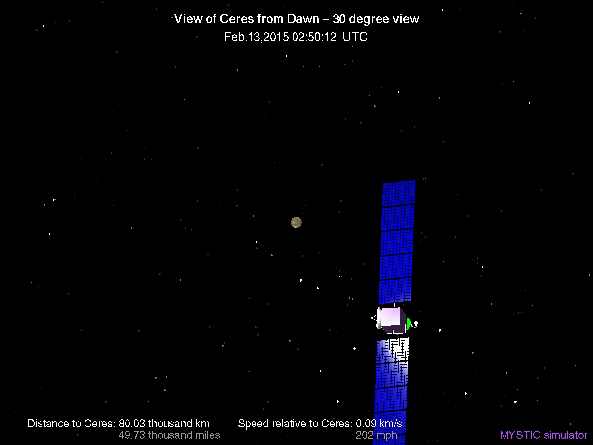
The JPL DAWN mission page has a button for Where is Dawn now?, which is in a drop-down menu if you click on Mission in the main menu on the left of the home page. Dawn of course is the spacecraft that visited the asteroid Vesta, and is now fast approaching Ceres.

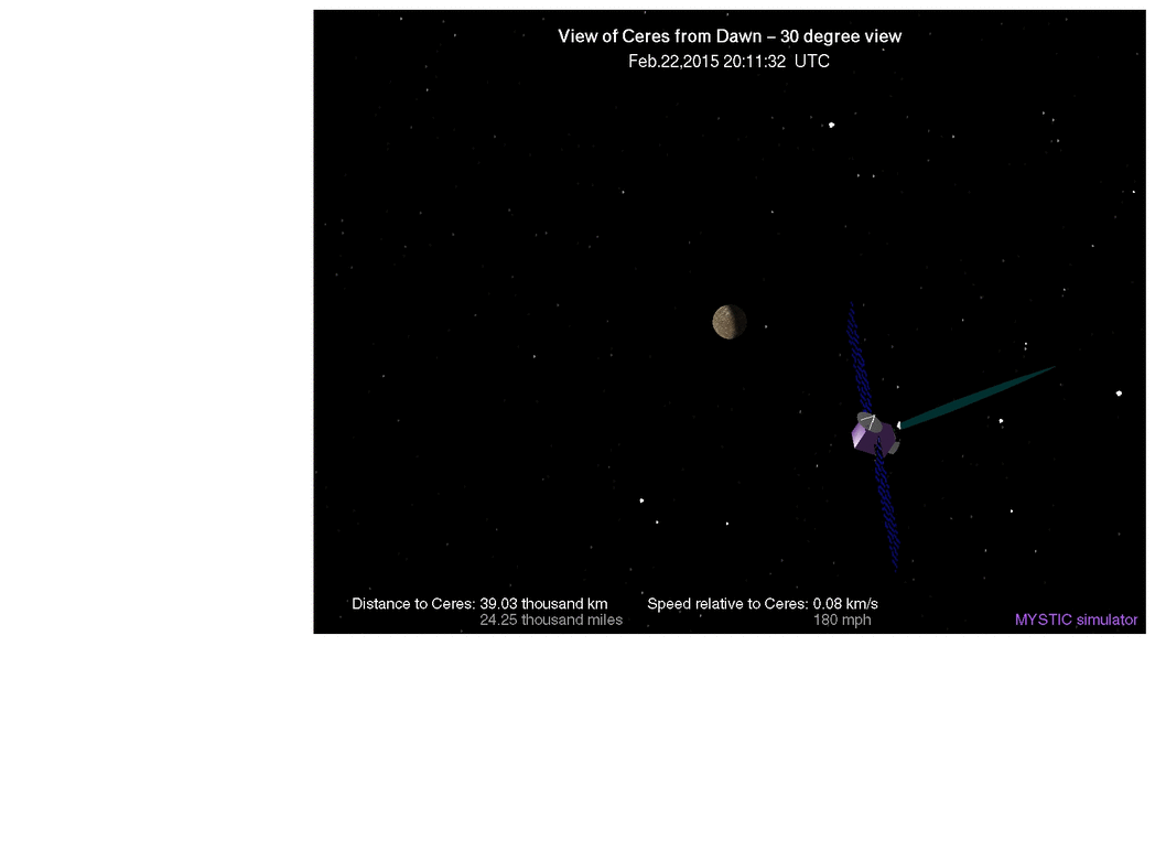
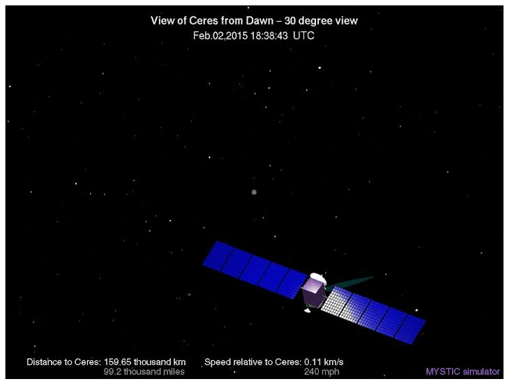
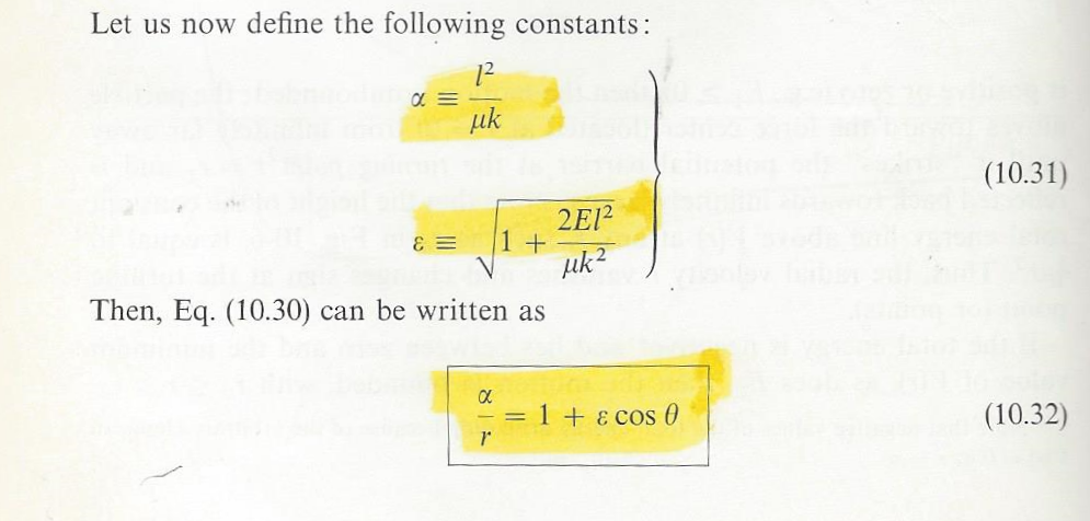
If you click on the graphic for Simulated View of Ceres from Dawn you get something like the following screen shot, from Feb 2, 2015
Feb02
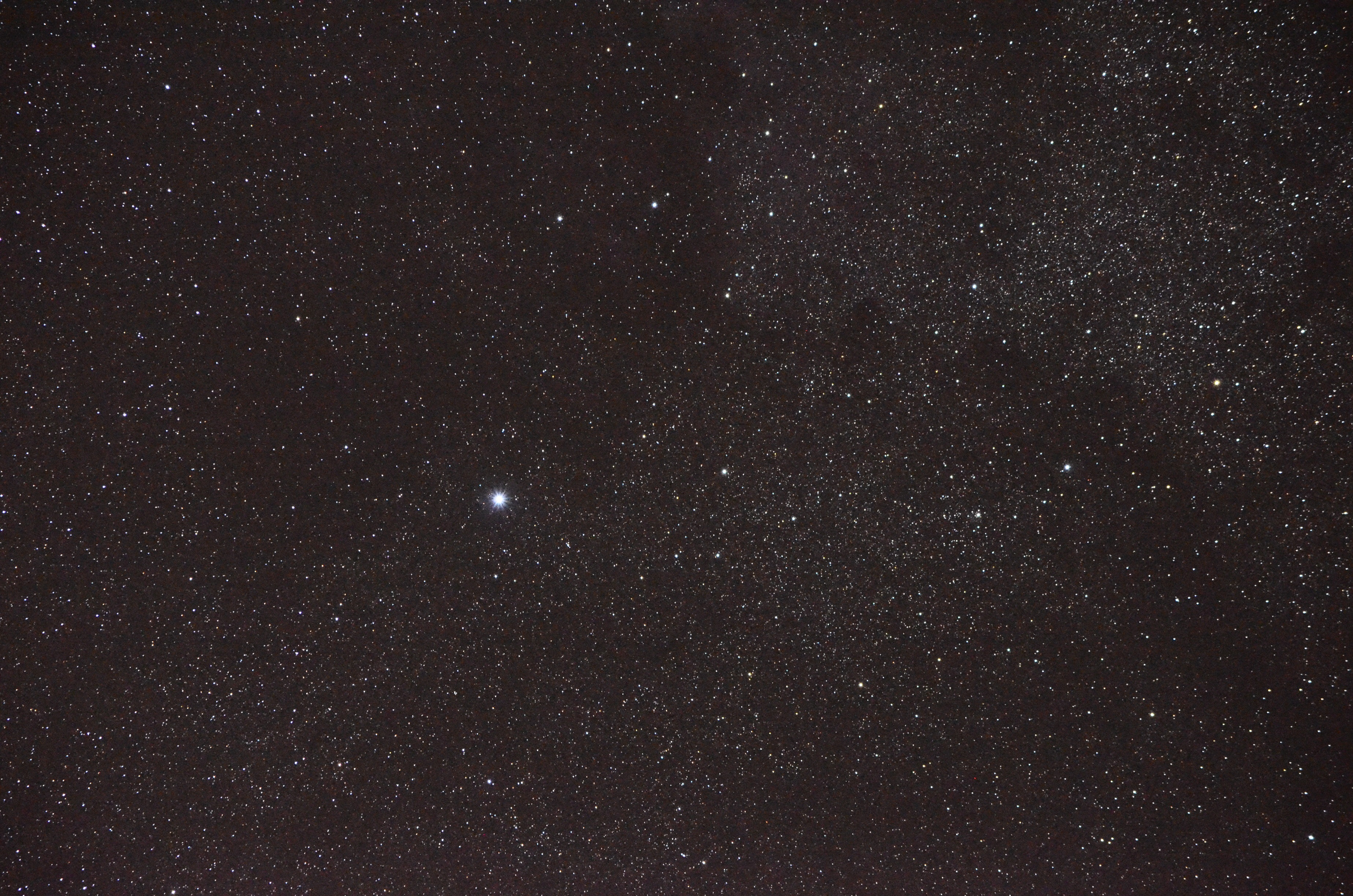
Well, this tells us that it is approaching Ceres, in the middle there, but what stars are those? I couldn’t recognize them, and it was driving me crazy. I thought if I tracked it for a while, I’d see something I recognized, but this got me nowhere.

Note the credit to MYSTIC simulator. This is a tool they hold pretty close to their vest. It is apparently very powerful and used in their actual trajectory planning. Searching for it, I found a link to the NASA/JPL SOLAR SYSTEM SIMULATOR, which is nice, but it provides a much different format, and I was not getting anywhere with it either. Since it was all I could use, I went back a year or so and looked at some wide fields of view, and I was able to track it back to the present, where the background was identifiable as being near the head of Draco, in our Northern sky, but I still had no luck correlating the stars to the MYSTIC image.

The reason for this, I finally realized, is that the SSS tool had not been kept up to date with the latest course corrections ( I presume ) as it gives a different distance from Ceres than MYSTIC, which is official, I guess.

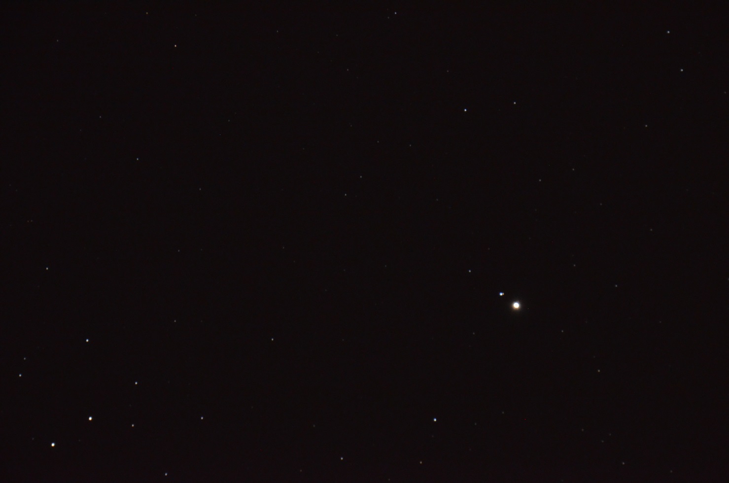
It was finally just dumb luck and persistence that enabled me to spot the correlating stars in my Starry Night software, and I’m sure you’ll agree it’s a good match:

output_DK8Cjt

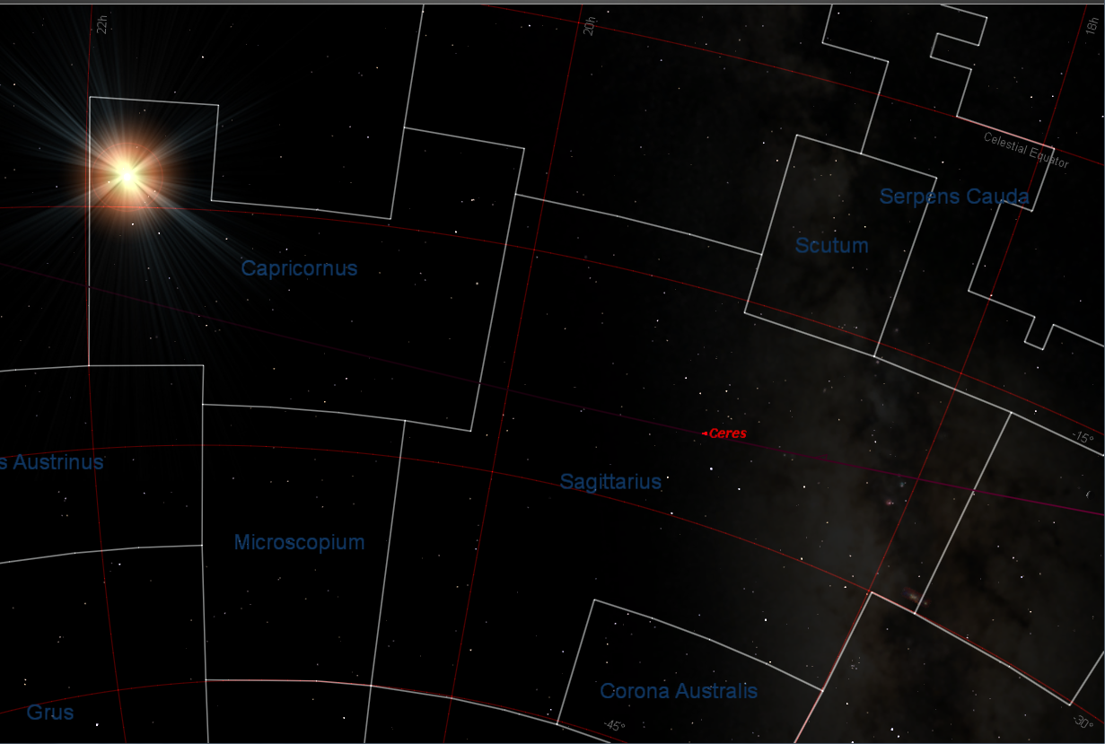
Note that the four stars of the almost-square “box” that Ceres is in ( and remained in for several days, ) is comprised of stars from three different constellations. Two in Serpens Cauda, and one each in Scutum and Ophiucus. A very obscure asterism !

Update: Feb 13

Here’s the latest WIDN image:Feb13

Ceres has “moved” ( in line of sight from DAWN ) “southward” ( in celestial coordinates ) into the constellation of Sagittarius. You might recognize the Sagittarian “teapot” asterism directly behind the bottom half of the representation of the DAWN space craft.

Now here’s the funny thing … DAWN is currently almost directly in line with Ceres from our terrestrial POV, as evidenced by this Starry Night view with Chicago set as the viewing location. Ceres is marked, along with it’s orbit. I adjusted the time to make the view align with the WIDN representation, and this view happens to occur at 9:46PM local time, on Feb 13, 2015. ( I did have to turn off the horizon mask, as this view is looking down through the ground at the given hour. Sagittarius rises just ahead of the sun at this season. )

I think this alignment has to be ascribed to coincidence, except that it does mean that DAWN is “rising” towards Ceres along an orbit which is “sunward” of Ceres’ orbit.

starry_Feb13_3

Update Feb 19

Here is an animated gif of a loosely spaced sequence of WIDN images, displaced to show a constant star background. This POV definitely gives the impression ( correct, I believe ) that DAWN is rising up through the ecliptic plane as it closes with Ceres. We can see Ceres sinking to the south below Sagittarius. It’s only going to get more interesting!output_4fYhUU

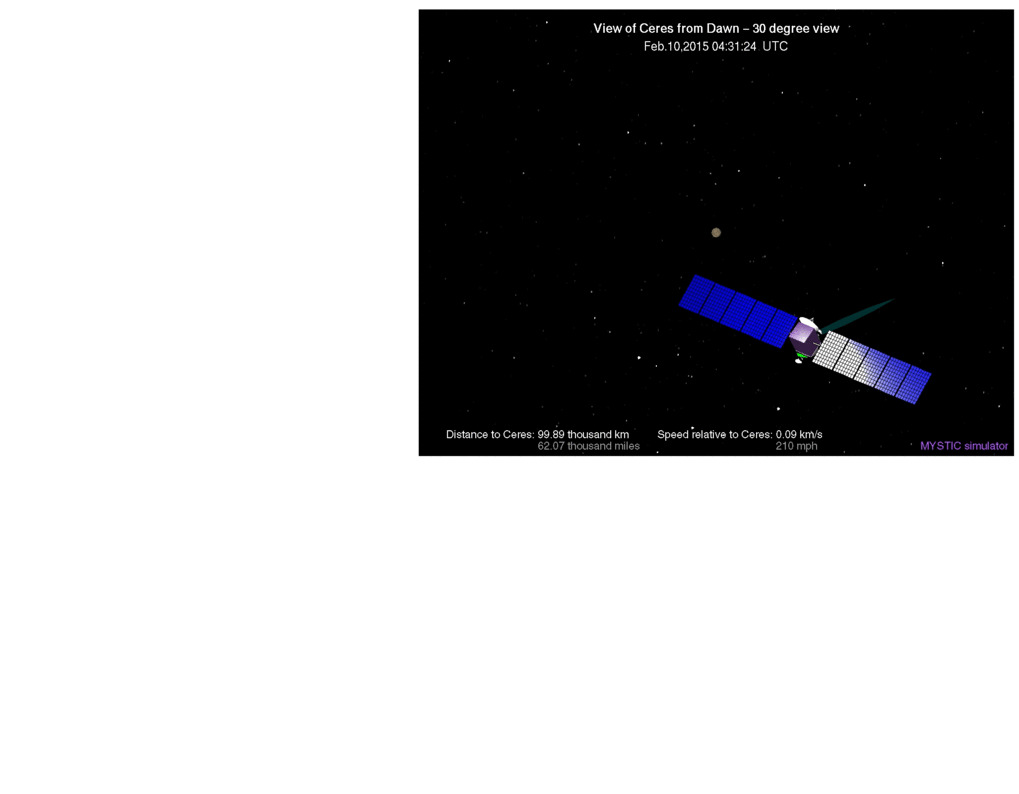
Feb 20 – A note on escape velocity

The Wikipedia article on Ceres gives a radius of 476 km and an escape velocity of .51 km/sec . This is the speed which gives an object a kinetic energy equal to the negative of the gravitational potential at this distance:

m v2/2 = m GM/R so v2/2 = GM/R

then the escape velocity at some r > R, say, is

vr = vR sqrt( R/r ) … very simple!

We note at Feb 20 03:16:52 we have r = 44580 km and v = .082 km/sec

but .51 km/sec sqrt(476/44580) = .053 km/sec

so DAWN is not gravitationally bound to Ceres at this point.

Note that the exact direction of the velocity is not important. Varying the direction just places the object with escape velocity at different places on various parabolic orbits.

Also note that the engine is not firing at this time. It seemed to be in braking mode the last few days, so has it shed any total energy?

On Feb 9 05:06:33 DAWN had r = 107010 km and v = .096 km/sec

The escape velocity at that distance is .51 km/sec sqrt(476/107010) = .034 km/sec

So the fact that it has shed considerable speed shows that it has gotten much closer to gravitational capture. If it were “drifting” it would have gained kinetic energy equal to the difference of the escape velocities at the two distances, requiring …

(v + delta_v )2 – v2 = .0532 – .0342

or v + delta_v = .104 km/sec

One more thing, braking with the same rocket is more effective at higher speeds, and one usually expects that a braking rocket will fire near close approach. The very low thrust of the ion rocket means that the approach has to be more “gentle”, which accounts for the braking having been in progress already. Let’s watch and see if DAWN does pick up a little more speed before the braking resumes, as it must.

… sure enough, DAWN is at 184 mph at Feb 20 13:22:16 vs. 182 mph at Feb 19 23:50:16
Kind of ironic that they give a more precise speed in mph vs. km/s, which is .08 for both times. 1 mph is ( exactly ) .00044704 km/s

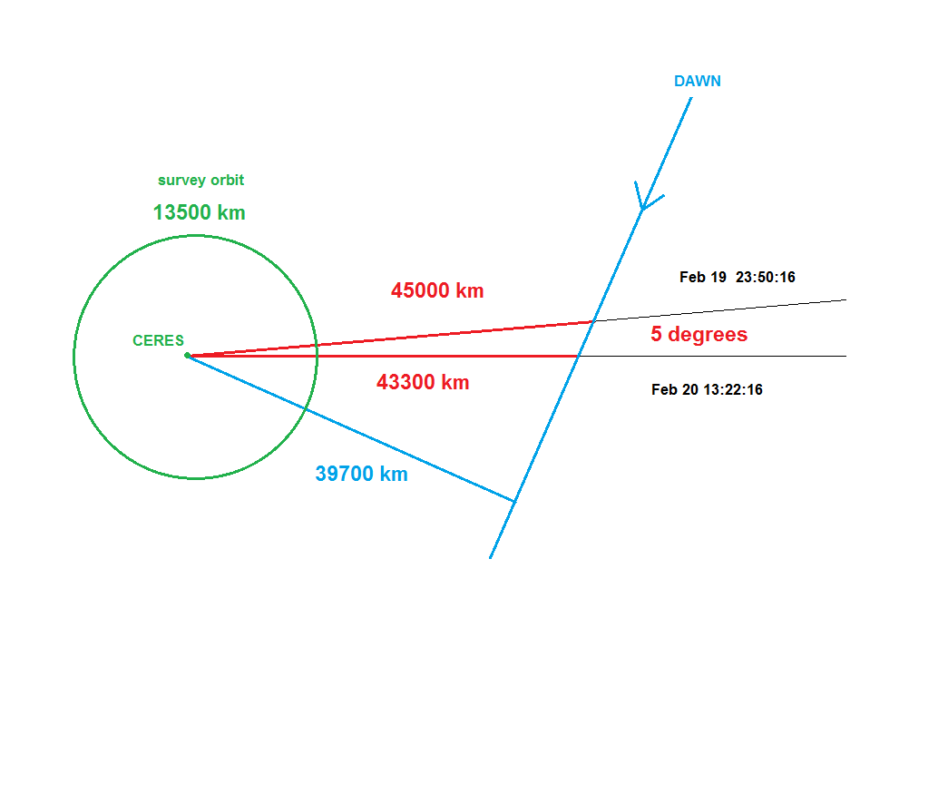
Feb 21 – The Approach Begins

Here’s a diagram I drew “by hand” in MS Paint showing the approach of DAWN to “Ceres Space” I started with the MYSTIC graphics for the times shown. I used the given distances and measured the angle of 5 degrees from the background stars, using my STARRY NIGHT software. This gave me the blue line and the close approach distance of a straight line trajectory.
draft

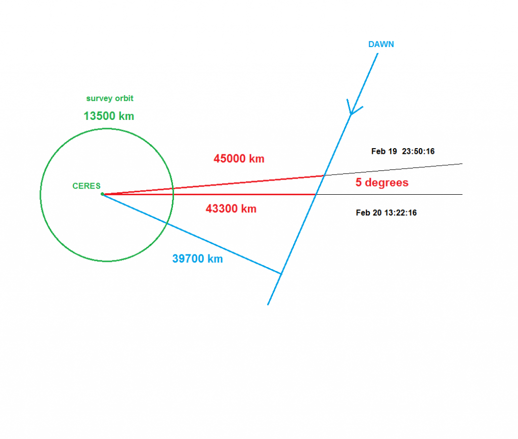
But what about the gravitational attraction of Ceres? It seems that DAWN is not yet bound to Ceres, but it should be on a discernible hyperbolic trajectory.

After some thrashing around with pencil and paper, I consulted my old copy of Marion’s CLASSICAL DYNAMICS and found the equation laid out for me, and highlighted to boot!
marion

I used my “hand built” yacc based calculator which features a plug-in definition capability. ( It actually pushes the defining string into the input stream when the defined symbol is encountered. )

Here are the defines I used:

define k “g*R^2”
define l “v*rp”
define alpha “l^2/k”
define E “v^2/2-k/r”
define e “(1+2*E*l^2/k^2)^0.5”

“mu”, for the “reduced mass” can be ignored when one body is much less massive than the other, m << M . Then mu ~= m and it cancels out of the expressions for alpha and e.

k is then GM, but I used GM/R2 = g to get k = g R2

Then setting the variables:
g= 0.00028
v= 0.083
rp= 39700
r= 45000
R= 476

( all in kilometers and seconds ) I just typed “alpha” and “e” to get the orbit parameters used in Marion’s equation 10.32, shown above:

alpha
1.71e+05
e
3.46

Then the distance of close approach and the angular displacement from the current position are given by:

alpha/(1+e)
3.84e+04
180/pi * acos( (alpha/r – 1)/e )
35.9

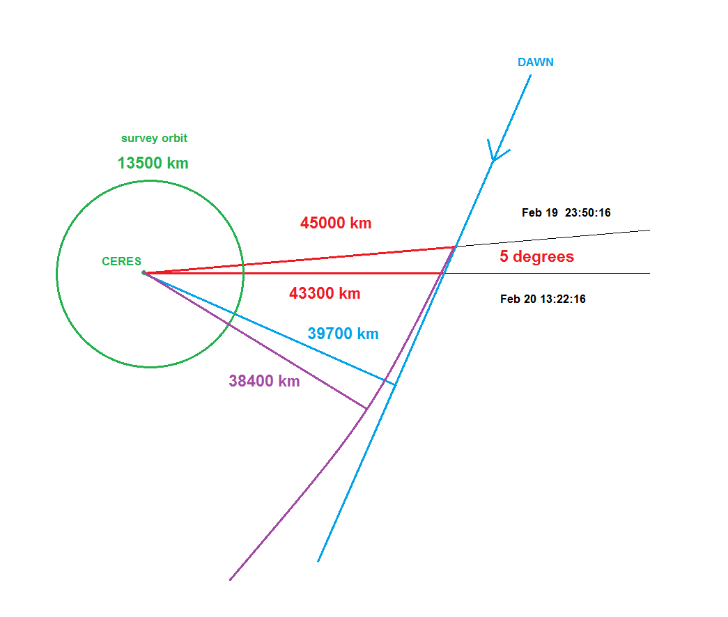
Perhaps surprisingly, these make sense! It says DAWN would approach to 38400 km at an angular displacement of 36 degrees from the current position, assuming it continued to “coast”.

Here’s the result roughly drawn in purple on the diagram. Of course, this is all in the realm of rough estimation!

orbit_diagram

ARE WE THERE YET ?

… Well, I say we are! According to a definite criterion that I will show you in this most recent animated gif: ( click to see the animation. )
output_81Cl4I

The bright star at top right is Fomalhaut in Piscis Austrinus. It’s actually visible on the southern horizon from mid-northern latitudes, but the POV is shifting to the south. and that’s the constellation Phoenix at the bottom.

But to make my point, I draw your attention to the “Distance to Ceres” caption at the bottom. Note that it “bottoms out” right at 24000 miles, and starts to increase again. DAWN is passing through “periceris” or whatever it might properly be termed. That is, a closest approach to Ceres. Of course, as it continues to “shed energy” it will spiral closer, but right now it is retaining the semblance of an hyperbolic orbit.

As we learned in physics class, the energy of a body at rest infinitely far from a gravitating body is conventionally set to ZERO. If it falls toward a gravitating body it gains kinetic energy but loses potential energy as it sinks into the “gravitational well”. So, any body with net positive energy can escape to infinity with a finite velocity, and is not bound to the gravitating body.

I say all this because the net energy of DAWN ( per unit mass ) is easy to calculate from the MYSTIC captions, and we can gauge its approach to gravitational binding by the steady diminishment that we see in this value, which is equal to 1/2 V_inf2, where V_inf is magnitude of the aforementioned “velocity at infinity”.

The value of V_inf was 115 mph in the last frame of the animation at Feb 24 06:33:54 . As of Feb 25 05:34:47, V_inf was down to 107 mph

March 10 – APOAPSIS

The “arrival” or attainment of zero orbital energy, was well noted on March 6, but there was nothing in the motion or actions of the DAWN spacecraft that would have indicated this event, such as it was. It has been “firing” its thruster steadily before during and after this milestone, as it continues to work towards its Survey Orbit. DAWN is now approaching another event, which has a more obvious connection to  its motion. That is apoapsis, as it is generically termed, or maybe apocerium, if we follow Kepler’s coinage of apohelium, which was later “greekified” to the now conventional aphelion.

As an aside, this question of what to call the “apo” point of the orbit has been bubbling along for decades, if not centuries. I only knew of aphelion and apogee, to be honest, but now I’m seeing that apoapsis, that is apo-apsis, is supposed to be the standard term, as awkward as it is. Investigating, I find that apogee derives from apogaeum, a nineteenth century analogue to Kepler’s apohelium, based on gaia, for the earth, I presume.

Of course, I became familiar with apogee from the era of “satellites” in the 50’s and 60’s, when I was quite young. I don’t see why the term can’t be applied to any planetary body, just as one speaks of Martian geology.

Well, at any rate, we are approaching the turning point of DAWN from its continuing motion away from Ceres ( despite it’s inevitable capture ) into a motion falling towards it. Following the Where Is Dawn Now? graphic on the DAWN mission page, we see that its motion is at a low point, suggesting a thrown object at its apex.. In the approximately six hours between Mar. 10,2015 00:03:54 and Mar. 10,2015 06:01:34, DAWN has decelerated from 78 mph to 76 mph, and moved 290 miles further from Ceres; from 43060 miles away to 43350 miles away. These are numbers appropriate to highway driving, not space travel!

So what happens when it “makes the turn” and starts falling towards Ceres ? I anticipate that they will turn off the thruster for a while and let it fall, but we’ll see.

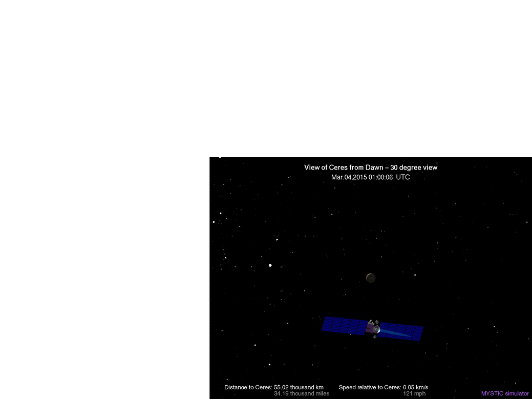
March 17 – Making the Turn

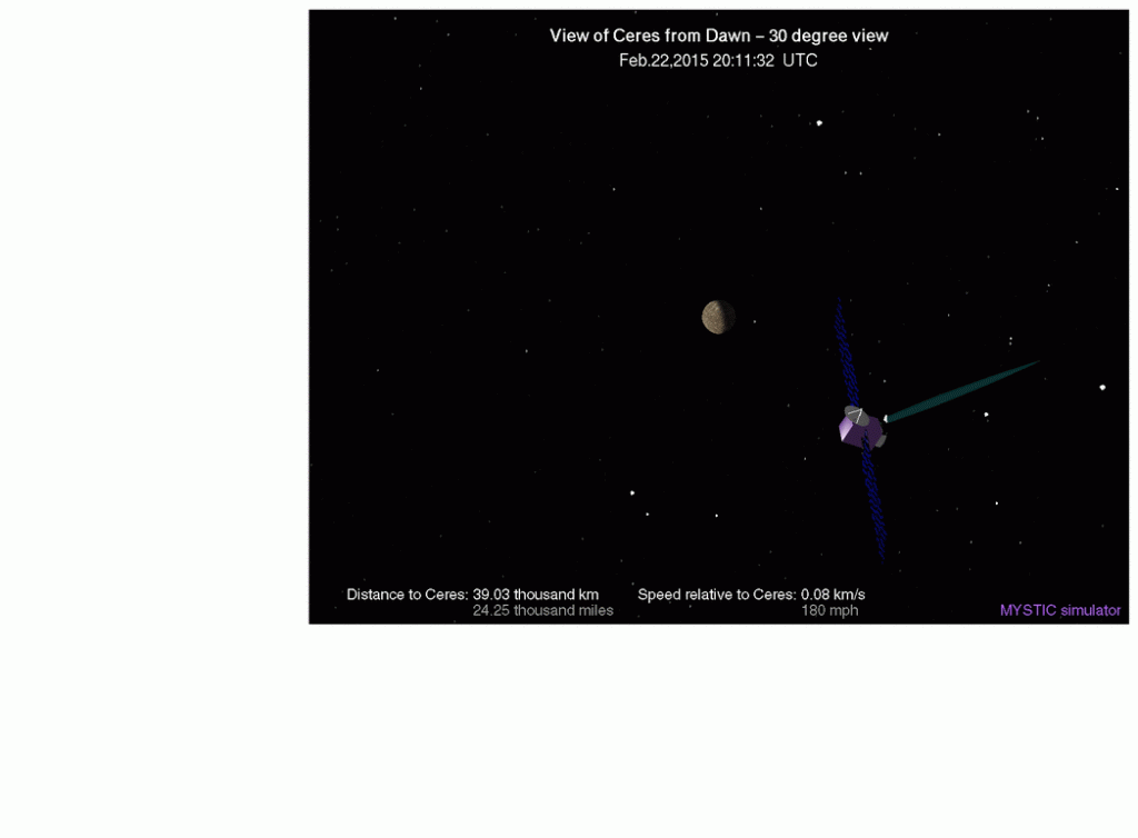
DAWN is still approaching apoapsis, but it is very near, as its speed relative to Ceres of a mere 40 mph would indicate. Here is an animated gif comprised of  1 frame per day for the 14 days March 4 thru March 17. I think you can see a slight bow in the arc of the apparent motion of Ceres against the constellation Orion as DAWN adjusts the plane of its orbit. I did the best I could to keep the star background constant, but its still not perfect, as you can see. I hope it’s good enough to allow you to picture the apparent motion of Ceres against the fixed stars from DAWN’s POV. The sun is almost coming into view just above Orion, as you can see by the almost completely dark disk of Ceres.

Note that the distance from Ceres increases from 55020 km to 77740 km during this interval as DAWN climbs to its apex. You can see the disk of Ceres diminish in size as DAWN recedes from it.

output_MbifyqMarch 25, 2015

On March 19 DAWN achieved apoapsis at 48740 miles from Ceres moving at 34 mph, and is now starting to move closer to Ceres. As of today at 10:33 UTC it has “fallen” to 46460 miles away, and is moving at 40 mph! Here we go!

BTW, DAWN is moving towards a point almost directly opposite the sun from Ceres. WHERE IS DAWN NOW? provides views of the sun ( and other objects ) from DAWN’s vantage point, and here is an overlay showing that the sun is just about to come into view in the Ceres frame of reference … along with the earth and mars too!

sun_Mar24_3

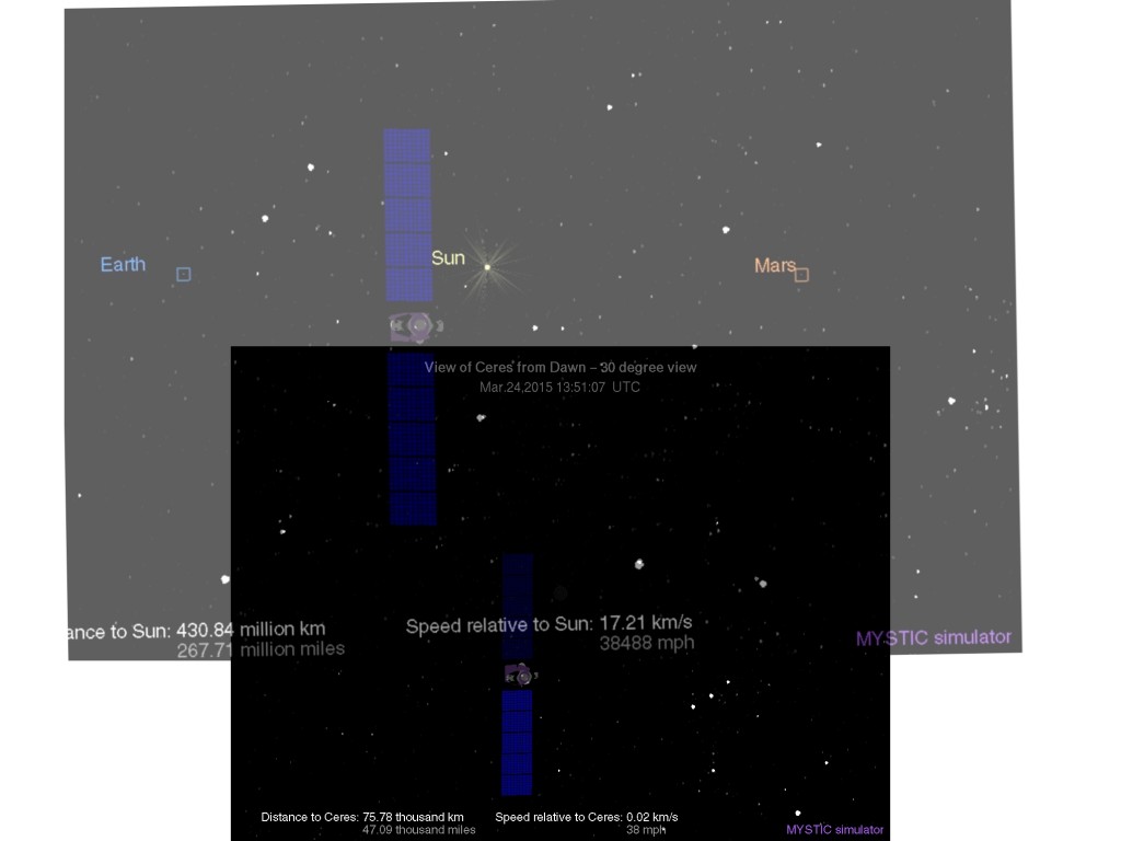
Note that I had to expand the “sun view” and slightly rotate it to get a matching overlay.


Rocket Science

The explosion of the Antares rocket carrying the ISS supplies on 10/28/2014 was a great disappointment, and a severe setback for the U.S. space program.

Nevertheless, it gets my sleuthing instinct up, which in this case involves some real background study on the Antares rocket.

Also, we have the development in the News of the idea, or “meme” if you will, that the “explosion” was due to a destruct signal.

This idea, which is quite typical of news developments, is distressing to me. It all hinges on rhetoric. In this case the rhetoric of the “kill signal” sent by the range safety officer, and also the identification of “the explosion” resulting thereto.

First reports of the destruct command gave the bare facts, that the range saftey officer had initiated it “before the rocket hit the ground”, but the report I read gave the specific qualification that it was not certain whether this signal accounted for the explosion.

By appearances, the authority of the range safety officer has prevailed in the news reports, so that we are now informed that the rocket “was destroyed in a massive explosion at the launch site after safety officers sent a kill signal.”

Against this idea, we may note that there were at least two explosions. An immediate explosion, apparently of an engine, within one second of the first visible anomaly, and the more famous and spectacular explosion as the rocket fell back to the launch pad. This second explosion is what is being promulgated in the news reports.

Here is an animated gif made from a rough division of the launch video obtained by “double taps” at my terminal. It spans approximately 2 seconds, as timed by the video.
output_g34UxB

Well, it simply defies credulity that the apparent explosion at the base of the rocket, in the vicinity of the engines ( there are two of them ) was initiated by a manual signal after the observation of the anomalous “flare” of the rocket plume. In fact, the “108 %” announcement is made right at this time, and verbal acknowledgement of the disaster is rather delayed.

So all I’m saying is that the 2 second interval labeled 4:14 thru 4:15 in this video is a true record of the “accident” itself. I don’t think this is particulary controversial, outside of the impression given by the news reports.

So then the question is, what happened? The flare indicates to me that there was a breach in the LOX circulation through the bell. Aside from the flare, this would have caused a drop in pressure, obviously, in the LOX feed to the engine, and to the turbine driving the pump. So things go south real fast with the flame front going “upstream” into the engine.

My conviction is that there are more than a few individuals on the development Orbital Sciences staff that knew immediately what had happened. The company has stated that the facts will be known in “days not weeks”, so any day now …